3D isosurfaces

Draws isosurfaces of a 3D scalar field, i.e. the surfaces on which the field equals given values. These are the 3D analog of contour lines, and can show the shape of a density, a concentration plume, an implicit surface, or any other function of three variables. Surfaces are triangulated with the marching cubes algorithm.

Usage

geom_isosurface_3d(
  mapping = NULL,
  data = NULL,
  stat = StatIsosurface3D,
  position = "identity",
  ...,
  levels = NULL,
  inside = "above",
  cap = FALSE,
  light = NULL,
  cull_backfaces = FALSE,
  scale_depth = TRUE,
  na.rm = FALSE,
  show.legend = NA,
  inherit.aes = TRUE
)

stat_isosurface_3d(
  mapping = NULL,
  data = NULL,
  geom = GeomIsosurface3D,
  position = "identity",
  ...,
  levels = NULL,
  inside = "above",
  cap = FALSE,
  light = NULL,
  cull_backfaces = FALSE,
  scale_depth = TRUE,
  na.rm = FALSE,
  show.legend = NA,
  inherit.aes = TRUE
)

Arguments

mapping: Set of aesthetic mappings created by aes().
data: The data to be displayed in this layer: a grid of points, with one row for every combination of x, y, and z values, such as produced by expand.grid(). Even grid spacing is not required.
stat: The statistical transformation to use on the data. Defaults to StatIsosurface3D.
position: Position adjustment, defaults to "identity". To collapse the result onto one 2D surface, use position_on_face().
...: Other arguments passed on to the layer function (typically GeomPolygon3D), such as aesthetics like colour, fill, linewidth, etc. Unless colour is mapped or set, opaque polygons are outlined in their fill color, which hides the seams between adjacent polygons, and translucent polygons aren't outlined. These outlines are lit along with the fill, whatever the fill and color arguments of light(). Contours and ridgelines are the exception, with outlines of their own.
levels: Numeric vector of values of the field at which to draw isosurfaces, one surface per value. Defaults to a single surface at the midpoint of the range of value.
inside: Which side of each surface is its inside, the region it encloses: "above" (the default) for where value exceeds the level, as for a density or concentration, or "below" for where it's less. Surfaces face outward from their insides, which determines where cap adds caps, which triangles cull_backfaces removes, and the direction of the computed normals.
cap: Logical indicating whether to close surfaces with flat caps where they meet the edges of the grid, or limits set on the plot's scales, so that they show solid cross sections rather than being left open there. Defaults to FALSE.
light: A lighting specification object created by light(), light("none") or the string "none" to disable lighting, or NULL to inherit plot-level lighting. Set plot-level lighting by adding light() to the plot, and layer-specific lighting via the light argument of geom_*_3d() functions, which takes precedence.
cull_backfaces: Logical indicating whether to remove triangles that face away from the viewer. Surfaces face outward from the regions they enclose, so for opaque surfaces that close on themselves, TRUE removes only hidden triangles and speeds up rendering. Defaults to FALSE, since surfaces that are translucent or cut open by the edge of the grid show their inner side.
scale_depth: Controls whether polygon linewidths are scaled to make closer lines wider and farther lines narrower, based on the mean depth of a polygon. TRUE (the default) applies full scaling and FALSE disables it; a number sets the strength directly, where 1 matches TRUE, 0 matches FALSE, values below 1 subdue the effect and values above 1 exaggerate it. This affects the layer only; use coord_3d(scale_depth = ) for gridlines, cube borders, axis ticks, and axis text.
na.rm: If FALSE, missing values are removed.
show.legend: Logical indicating whether this layer should be included in legends.
inherit.aes: If FALSE, overrides the default aesthetics.
geom: The geometric object used to display the data. Defaults to GeomIsosurface3D, a variant of geom_polygon_3d().

Value

A Layer object that can be added to a ggplot.

Details

Where limits are set on the plot's scales, e.g. with ggplot2::xlim() or zlim(), surfaces are cut at the last grid points within the limits, leaving them open there unless cap = TRUE.

Aesthetics

stat_isosurface_3d() requires the following aesthetics:

x, y, z: Grid point coordinates
value: The value of the field at each grid point

Grouping aesthetics give separate fields, each needing its own complete grid.

geom_isosurface_3d() understands the same aesthetics as geom_polygon_3d(). Unless color is mapped or set, opaque triangles are outlined in their fill color, which hides seams between them, and translucent triangles (alpha below 1) are not outlined.

Computed variables

level: The value of the field on the surface
normal_x, normal_y, normal_z: Components of each triangle's unit normal, pointing outward from the region the surface encloses (see inside)
cap: Whether a triangle is part of a cap (see cap), e.g. for aes(fill = after_stat(cap))

Dependencies

Isosurfaces are computed with the rmarchingcubes package, which must be installed.

Examples

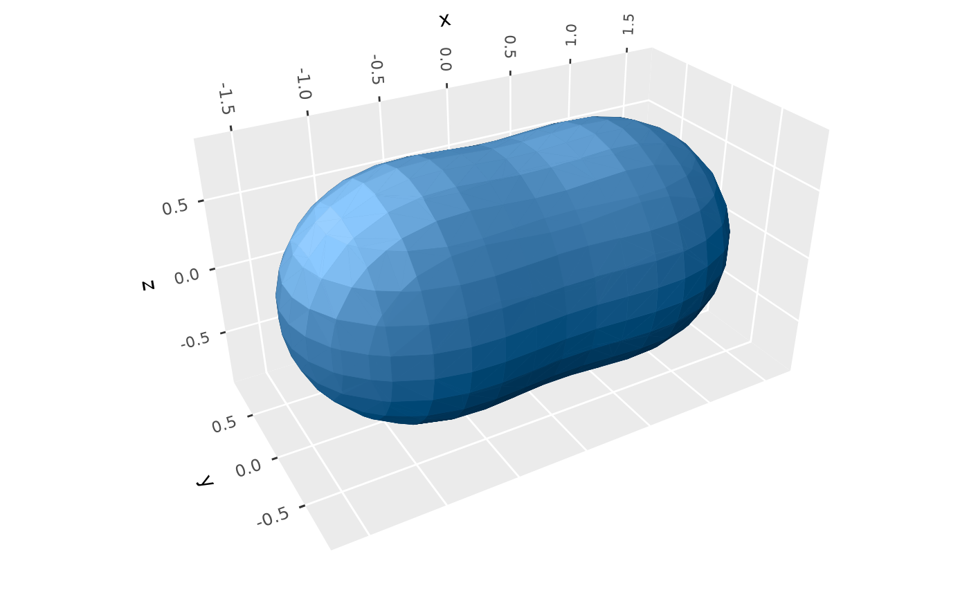
# A field with two peaks
blobs <- expand.grid(x = seq(-2.5, 2.5, length.out = 24),
                     y = seq(-2, 2, length.out = 24),
                     z = seq(-2, 2, length.out = 24))
blobs$value <- with(blobs, exp(-((x - 0.8)^2 + y^2 + z^2)) +
                           exp(-((x + 0.8)^2 + y^2 + z^2)))

# A single surface, by default at the midpoint of the value range
ggplot(blobs, aes(x, y, z, value = value)) +
  geom_isosurface_3d(fill = "steelblue") +
  coord_3d(scales = "fixed")


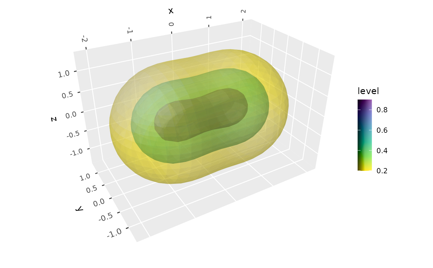
# Nested translucent surfaces, colored by level
ggplot(blobs, aes(x, y, z, value = value, fill = after_stat(level))) +
  geom_isosurface_3d(levels = c(0.2, 0.5, 0.9), alpha = 0.4) +
  scale_fill_viridis_c(direction = -1) +
  coord_3d(scales = "fixed")


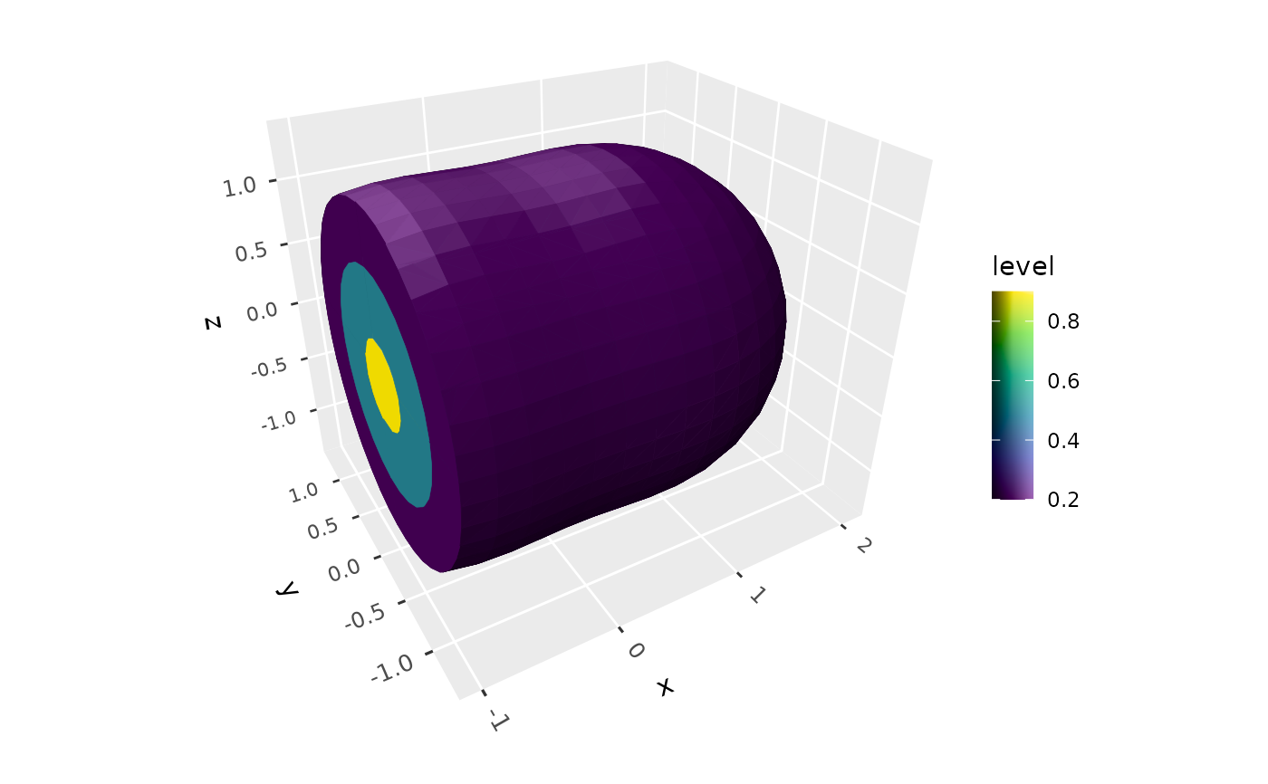
# \donttest{
# Cut by a limit, with caps showing the cross section
ggplot(blobs, aes(x, y, z, value = value, fill = after_stat(level))) +
  geom_isosurface_3d(levels = c(0.2, 0.5, 0.9), cap = TRUE) +
  scale_fill_viridis_c() +
  xlim(-1, NA) +
  coord_3d(scales = "fixed")
#> Warning: Removed 4032 rows containing non-finite outside the scale range
#> (`stat_isosurface3d()`).


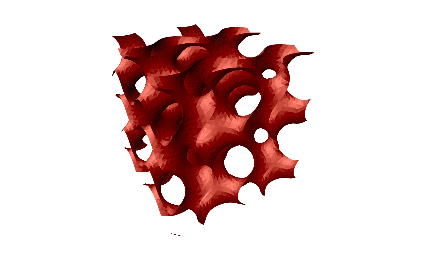
# An implicit surface: the gyroid, sin(x)cos(y) + sin(y)cos(z) + sin(z)cos(x) = 0
gyroid <- expand.grid(x = seq(0, 4 * pi, length.out = 40),
                      y = seq(0, 4 * pi, length.out = 40),
                      z = seq(0, 4 * pi, length.out = 40))
gyroid$value <- with(gyroid, sin(x) * cos(y) + sin(y) * cos(z) + sin(z) * cos(x))

ggplot(gyroid, aes(x, y, z, value = value)) +
  geom_isosurface_3d(levels = 0.5, fill = "darkred") +
  coord_3d(panels = "none") +
  theme_void()

# }