geom_polygon_3d() renders 3D polygons with proper depth sorting for realistic
3D surface visualization. It's designed to work with surface data
from stat_hull_3d() and stat_surface_3d(), as well as regular polygon data like maps.
Usage
geom_polygon_3d(
  mapping = NULL,
  data = NULL,
  stat = StatIdentity3D,
  position = "identity",
  ...,
  rule = "evenodd",
  sort_method = "auto",
  scale_depth = TRUE,
  force_convex = FALSE,
  cull_backfaces = FALSE,
  light = NULL,
  na.rm = FALSE,
  show.legend = NA,
  inherit.aes = TRUE
)
Arguments
- mapping
Set of aesthetic mappings created by
aes().- data
The data to be displayed in this layer. Note that if you specify
lightorcull_backfaces, behavior will depend on the "winding order" of polygon vertices, with the counter-clockwise face considered the "front".- stat
The statistical transformation to use on the data. Defaults to
"identity_3d".- position
Position adjustment, defaults to "identity". To collapse the result onto one 2D surface, use
position_on_face().- ...
Other arguments passed on to the layer function (typically GeomPolygon3D), such as aesthetics like
colour,fill,linewidth,annotate = annotate_3d(...), etc.- rule
Either
"evenodd"or"winding". If polygons with holes are being drawn (using thesubgroupaesthetic) this argument defines how the hole coordinates are interpreted. Seeggplot2::geom_polygon()for reference.- sort_method
Depth sorting algorithm. See sorting_methods for details.
- scale_depth
Logical indicating whether polygon linewidths should be scaled to make closer lines wider and farther lines narrower. Default is TRUE. Scaling is based on the mean depth of a polygon.
- force_convex
Logical indicating whether to remove polygon vertices that are not part of the convex hull. Default value varies by geom. Specifying TRUE can help reduce artifacts in surfaces that have polygon tiles that wrap over a visible horizon. For prism-type geoms like columns and voxels, FALSE is safe because polygons fill always be convex.
- cull_backfaces
Logical indicating whether to remove back-facing polygons from rendering. This is primarily for performance optimization but may be useful for aesthetic reasons in some situations. Backfaces are determined using screen-space winding order after 3D transformation. Defaults vary by geometry type: FALSE for open surface-type geometries, TRUE for solid objects (hulls, voxels, etc. where backfaces are generally hidden unless frontfaces are transparent or explicitly disabled).
- light
A lighting specification object created by
light(),"none"to disable lighting, orNULLto inherit plot-level lighting specs from the coord. Specify plot-level lighting incoord_3d()and layer-specific lighting ingeom_*3d()functions.- na.rm
If
FALSE, missing values are removed.- show.legend
Logical indicating whether this layer should be included in legends.
- inherit.aes
If
FALSE, overrides the default aesthetics.
Aesthetics
geom_polygon_3d() requires:
x: X coordinate
y: Y coordinate
z: Z coordinate (for depth sorting)
group: Polygon grouping variable
And understands these additional aesthetics:
fill: Polygon fill colorcolour: Border colorlinewidth: Border line widthlinetype: Border line typealpha: Transparencysubgroup: Secondary grouping for polygons with holesorder: Vertex order within polygons (for proper polygon construction)
Examples
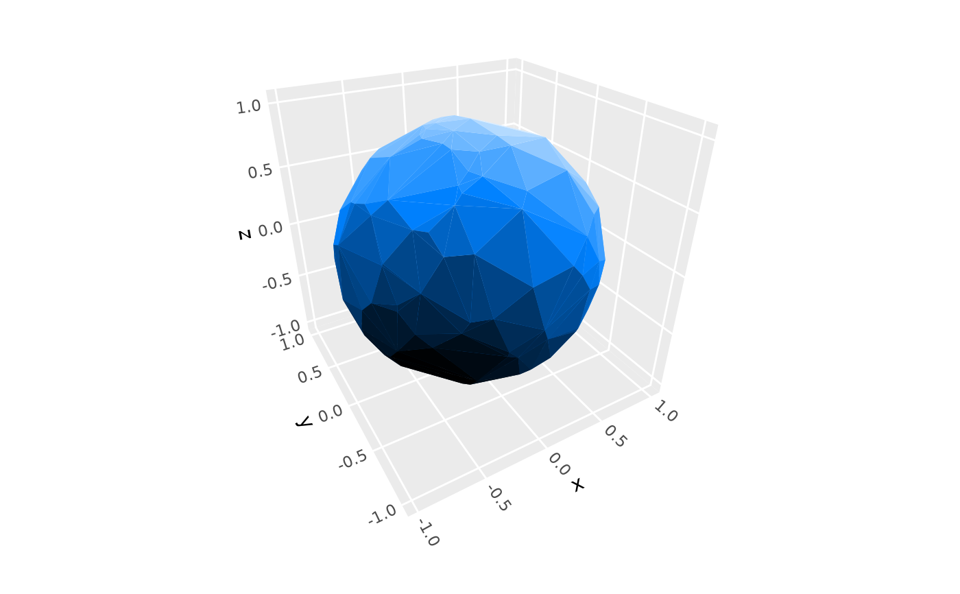
# Typically used via stats such as stat_surface_3d() or stat_hull_3d()
ggplot(sphere_points, aes(x, y, z)) +
stat_hull_3d(method = "convex", fill = "dodgerblue",
light = light(fill = TRUE, mode = "hsl")) +
coord_3d()
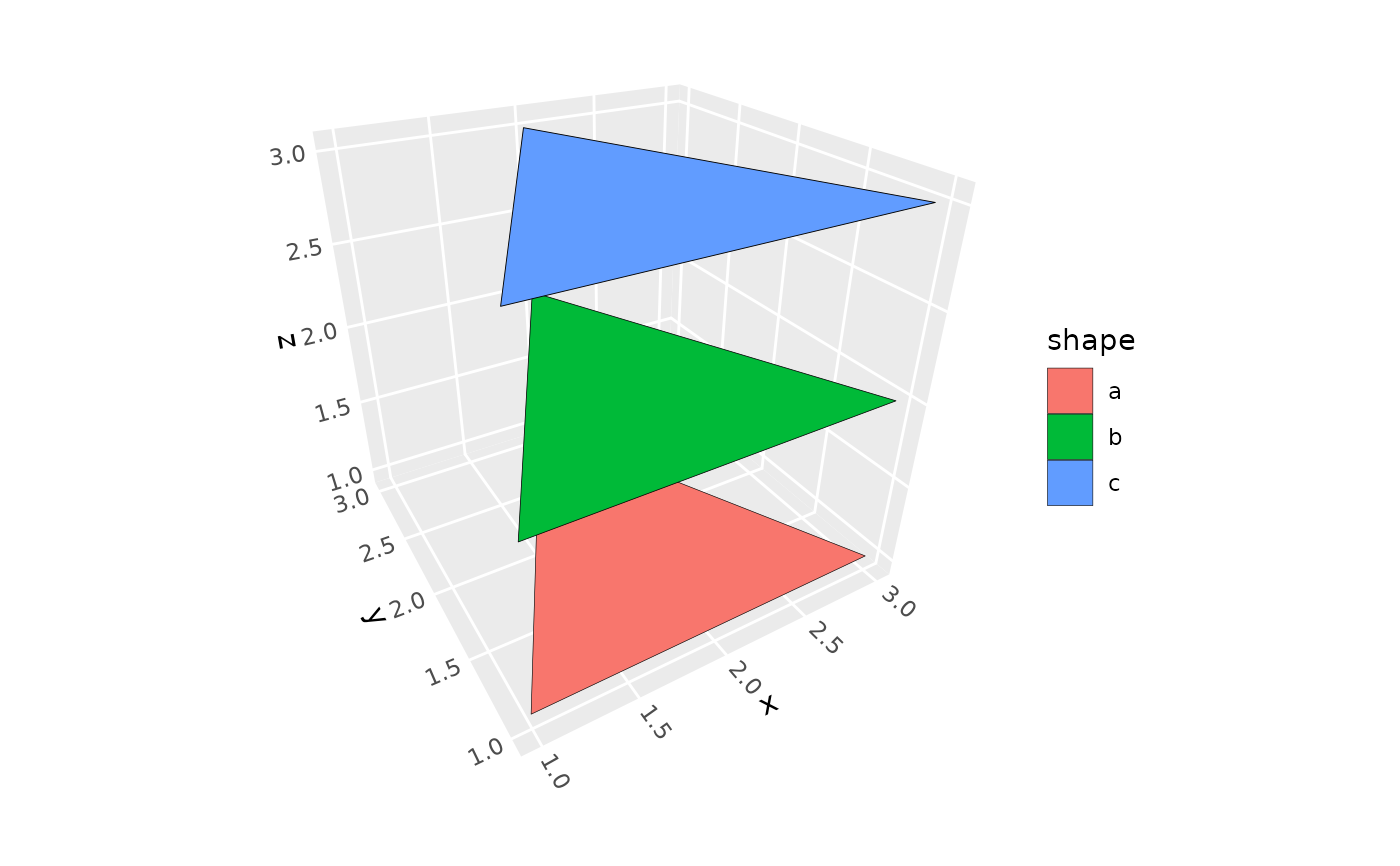
 # Can be used directly with properly structured data
triangles <- data.frame(x = rep(c(3, 2, 1), 3),
y = rep(c(1, 3, 1), 3),
z = rep(1:3, each = 3),
shape = rep(letters[1:3], each = 3))
ggplot(triangles, aes(x, y, z, fill = shape)) +
geom_polygon_3d(color = "black") +
coord_3d()
# Can be used directly with properly structured data
triangles <- data.frame(x = rep(c(3, 2, 1), 3),
y = rep(c(1, 3, 1), 3),
z = rep(1:3, each = 3),
shape = rep(letters[1:3], each = 3))
ggplot(triangles, aes(x, y, z, fill = shape)) +
geom_polygon_3d(color = "black") +
coord_3d()
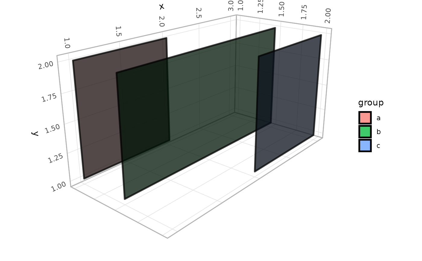
 # Use `sort_method` to choose between depth sorting algorithms
d <- data.frame(group = rep(letters[1:3], each = 4),
x = c(1, 1, 2, 2, 1, 1, 3, 3, 2, 2, 3, 3),
y = rep(c(1, 2, 2, 1), 3),
z = rep(c(1, 1.5, 2), each = 4))
p <- ggplot(d, aes(x, y, z, group = group, fill = group)) +
coord_3d(pitch = 50, roll = 20, yaw = 0,
scales = "fixed", light = "none") +
theme_light()
# fast, but rendering order is incorrect in this particular example
p + geom_polygon_3d(color = "black", linewidth = 1, alpha = .75,
sort_method = "painter")
# Use `sort_method` to choose between depth sorting algorithms
d <- data.frame(group = rep(letters[1:3], each = 4),
x = c(1, 1, 2, 2, 1, 1, 3, 3, 2, 2, 3, 3),
y = rep(c(1, 2, 2, 1), 3),
z = rep(c(1, 1.5, 2), each = 4))
p <- ggplot(d, aes(x, y, z, group = group, fill = group)) +
coord_3d(pitch = 50, roll = 20, yaw = 0,
scales = "fixed", light = "none") +
theme_light()
# fast, but rendering order is incorrect in this particular example
p + geom_polygon_3d(color = "black", linewidth = 1, alpha = .75,
sort_method = "painter")
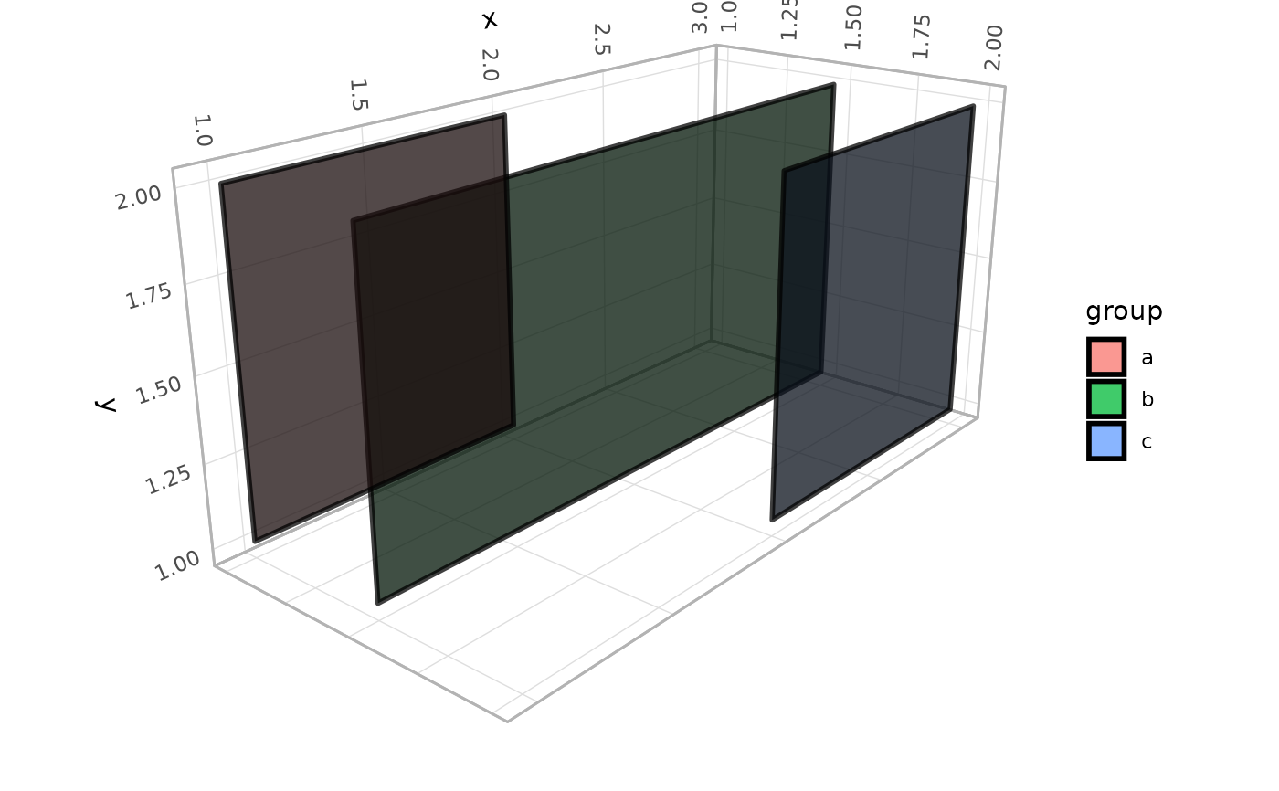 # correct rendering order (but slower for large data sets)
p + geom_polygon_3d(color = "black", linewidth = 1, alpha = .75,
sort_method = "pairwise")
# correct rendering order (but slower for large data sets)
p + geom_polygon_3d(color = "black", linewidth = 1, alpha = .75,
sort_method = "pairwise")