Because ggcube renders a 3D scene from a fixed camera angle, a single
plot only ever shows one viewpoint. Two functions let you show more than
one: animate_3d() moves the camera through a sequence of
angles and plays them back as a GIF or movie, while
orbit_3d() renders the same kind of sequence (or a 2D grid
of rotation angles) into a HTML “orbit” widget you can drag to
rotate.
Animations and orbits can be displayed in RStudio’s viewer, exported and viewed in a web browser, added to Shiny apps, or knit into RMarkdown documents like Reveal.js presentations or pkgdown articles.
Both functions simply render the plot many times at different rotations, so they preserve ggcube’s exact look — every frame is a real ggcube render, with the same lighting, depth sorting, and color scales.
The two functions share a rotation vocabulary. They operate on a
pre-existing ggcube plot object, and take pitch,
roll, and yaw arguments that define rotation
ranges to move through.
We’ll use a common base plot throughout this article – an alpha hull of points from a mammoth skeleton digitized by the Smithsonian:
mammoth <- data.frame(do.call(rbind, rjson::fromJSON(
file = paste0("https://raw.githubusercontent.com/PAIR-code/",
"understanding-umap/master/raw_data/mammoth_3d_50k.json")
)))
colnames(mammoth) <- c("Y", "X", "Z")
p <- ggplot(mammoth, aes(X, Y, Z)) +
geom_hull_3d(method = "alpha", radius = 8,
fill = "darkred", color = "darkred") +
light(mode = "hsl", direction = c(-1, 1, 0), anchor = "camera") +
coord_3d(roll = -90, scales = "fixed", zoom = 1.1,
panels = "zmin", expand = FALSE) +
theme(axis.text = element_blank(),
axis.ticks = element_blank(),
axis.title = element_blank())Animations
animate_3d() takes a plot and a set of keyframe angles,
interpolates between them, and renders the frames into an animation.
Each of pitch, roll, and yaw is
either held at a single value or given as a vector of keyframes to move
through; the camera is linearly interpolated between successive
keyframes.
The most common case is a turntable spin — a full yaw
rotation, holding the other angles fixed. nframes sets the
number of rendered frames and fps the playback speed:
animate_3d(p, yaw = c(0, 360), nframes = 60, fps = 10, width = 700)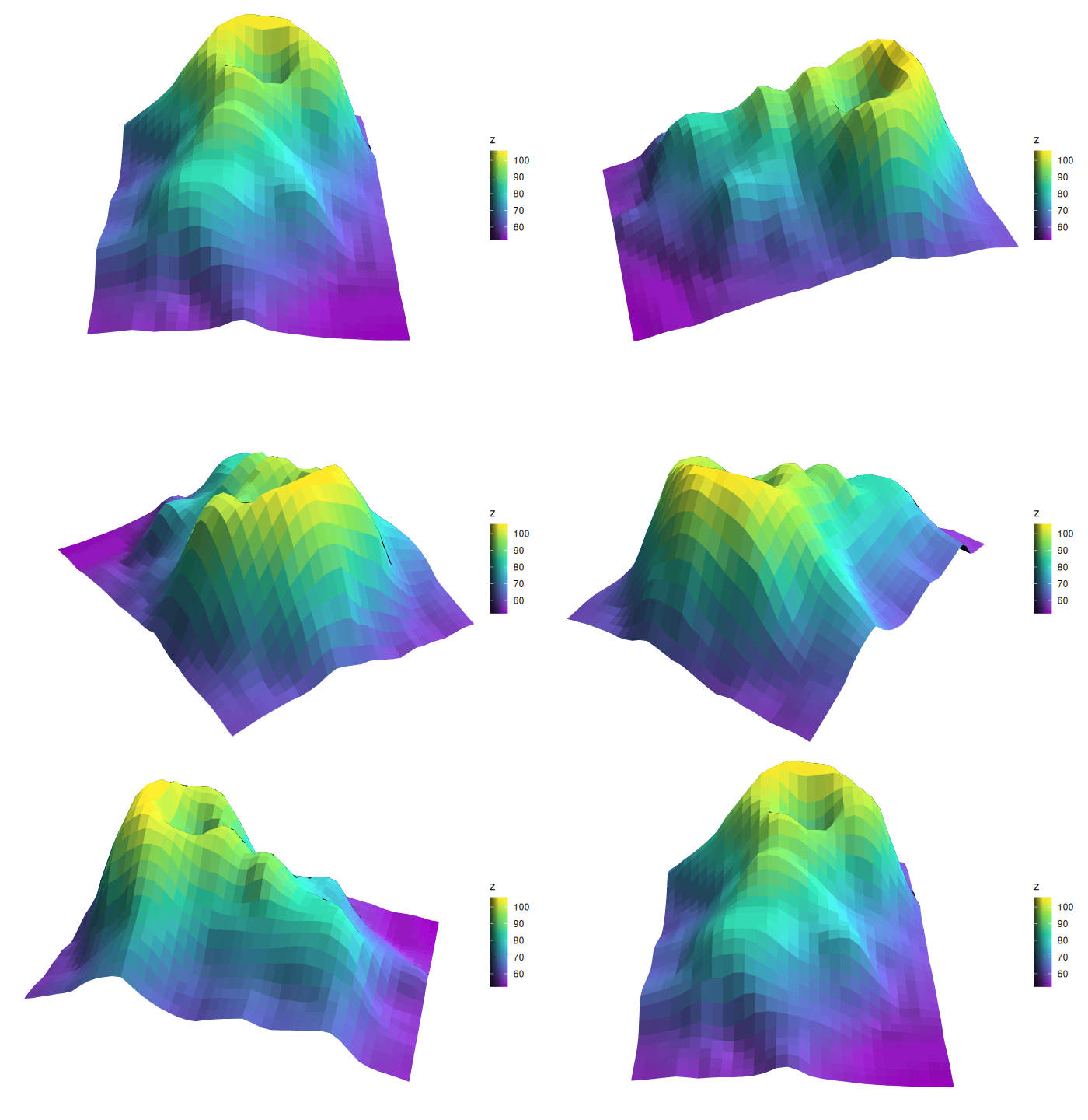
Keyframes can also trace a more complex path. Here the view moves
through several angles on two axes at once, tilting on the
roll axis while it spins in yaw:
animate_3d(p,
yaw = c(0, 720),
roll = c(-90, 0, -90),
nframes = 120, fps = 10, width = 700)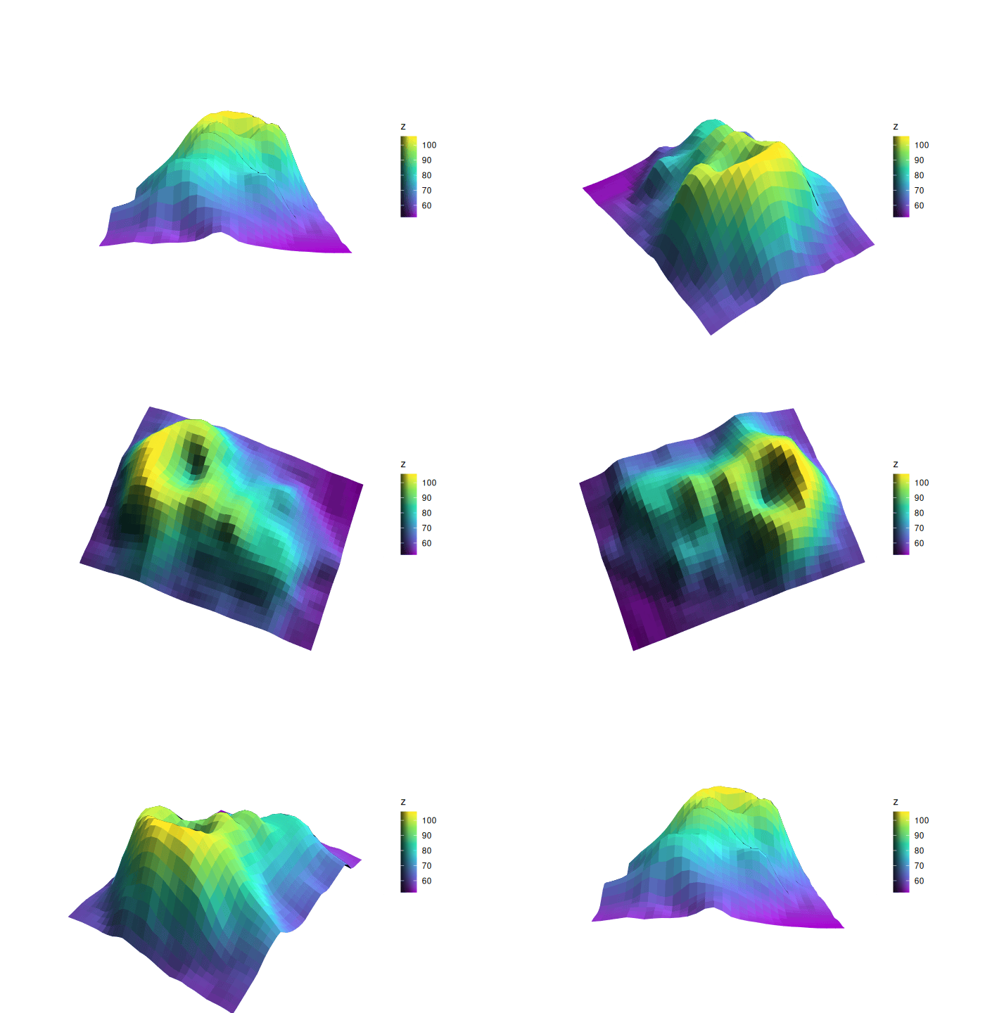
By default the animation is written to a temporary file and
displayed, but you can use file = to save it.
See ?animate_3d for the full set of playback options,
including frame timing, pauses, rewind, alternative renderers, and
parallel rendering.
Interactive orbits
orbit_3d() also renders a set of plots at different
rotation angles, but it instead packages the frames into an interactive
HTML widget that you can drag to rotate. Clicking and dragging with your
cursor, or using your keyboard arrow keys (after clicking or
tab-selecting the plot), changes the viewing angle.
Rotation is specified the same way as in animation, except that here
each angle is given as a range rather than a keyframe path. Specifying
the range in ascending vs. descending order switches the control
direction; note that for yaw specifically, specifying the
larger angle first (e.g. c(360, 0)) is generally preferred
so that rotation direction matches drag direction.
Full-turn ranges (e.g. yaw = c(0, 360)) wrap around
seamlessly, so you can keep dragging in one direction forever, while
partial ranges stop at their endpoints. Use start = to
choose the initial angle. Smoothness is governed by the frame count
n, with the trade-off that more frames take longer to
render and produce larger files.
Specifying a single range gives a 1D orbit or turntable effect — drag left and right to spin it:
For a 2D orbit, you specify two ranges; horizontal drag turns the
plot on one axis and vertical drag on the other, letting you both spin
and tilt the plot. The two numbers in n set the resolution
of each axis, and their product determines the number of rendered
frames, so keep them modest: