3D surface from regular grid data

Creates 3D surfaces from regularly gridded data (like elevation maps). The data must be on a regular, complete grid where every combination of x and y values appears exactly once.

Usage

geom_surface_3d(
  mapping = NULL,
  data = NULL,
  stat = StatSurface3D,
  position = "identity",
  ...,
  grid = "quad",
  light = NULL,
  cull_backfaces = FALSE,
  sort_method = NULL,
  force_convex = TRUE,
  scale_depth = TRUE,
  na.rm = FALSE,
  show.legend = NA,
  inherit.aes = TRUE
)

stat_surface_3d(
  mapping = NULL,
  data = NULL,
  geom = GeomPolygon3D,
  position = "identity",
  ...,
  grid = "quad",
  light = NULL,
  cull_backfaces = FALSE,
  sort_method = NULL,
  force_convex = TRUE,
  scale_depth = TRUE,
  na.rm = FALSE,
  show.legend = NA,
  inherit.aes = TRUE
)

Arguments

mapping: Set of aesthetic mappings created by aes(). This stat requires the x, y, and z aesthetics.
data: The data to be displayed in this layer. Must contain x, y, z columns representing coordinates on a regular grid.
stat: The statistical transformation to use on the data. Defaults to StatSurface3D.
position: Position adjustment, defaults to "identity". To collapse the result onto one 2D surface, use position_on_face().
...: Other arguments passed on to the the layer function (typically GeomPolygon3D), such as aesthetics like colour, fill, linewidth, etc.
grid: Character specifying desired surface grid geometry: either "quad" (the default) for a rectangular grid, "tri1" for a grid of right triangles with diagonals running in one direction, or "tri2" for a grid of right triangles with the opposite orientation. Triangles produce a proper 3D surface that can prevent lighting artifacts in places where a surface curves past parallel with the sight line.
light: A lighting specification object created by light() (see that function for details), or NULL to disable shading. Specify plot-level lighting in coord_3d() and layer-specific lighting in geom_*3d() functions.
cull_backfaces, sort_method, force_convex, scale_depth: Advanced polygon rendering parameters. See polygon_rendering for details.
na.rm: If FALSE, missing values are removed.
show.legend: Logical indicating whether this layer should be included in legends.
inherit.aes: If FALSE, overrides the default aesthetics.
geom: The geometric object used to display the data. Defaults to GeomPolygon3D.

Value

A Layer object that can be added to a ggplot.

Aesthetics

Requires the following aesthetics:

x: X coordinate
y: Y coordinate
z: Z coordinate (elevation/height)

Computed variables

The following computed variables are available via after_stat():

x, y, z: Grid coordinates and function values
normal_x, normal_y, normal_z: Surface normal components
slope: Gradient magnitude from surface calculations
aspect: Direction of steepest slope from surface calculations
dzdx, dzdy: Partial derivatives from surface calculation

Examples

# simulated data and base plot for basic surface
d <- dplyr::mutate(tidyr::expand_grid(x = -10:10, y = -10:10),
      z = sqrt(x^2 + y^2) / 1.5,
      z = cos(z) - z)
p <- ggplot(d, aes(x, y, z)) + coord_3d()

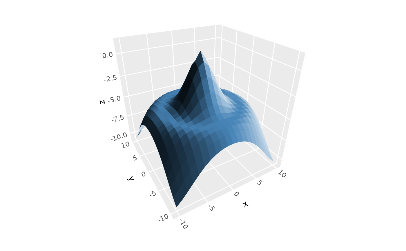
# surface with 3d lighting
p + geom_surface_3d(fill = "steelblue", color = "steelblue", linewidth = .2,
      light = light(mode = "hsl", direction = c(1, 0, 0)))


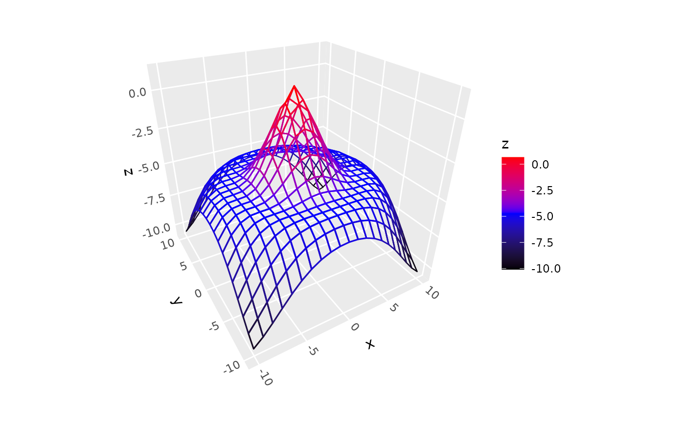
# mesh wireframe (`fill = NULL`) with aes line color
p + geom_surface_3d(aes(color = z), fill = NA,
      linewidth = .5, light = light(color = FALSE)) +
  scale_color_gradientn(colors = c("black", "blue", "red"))


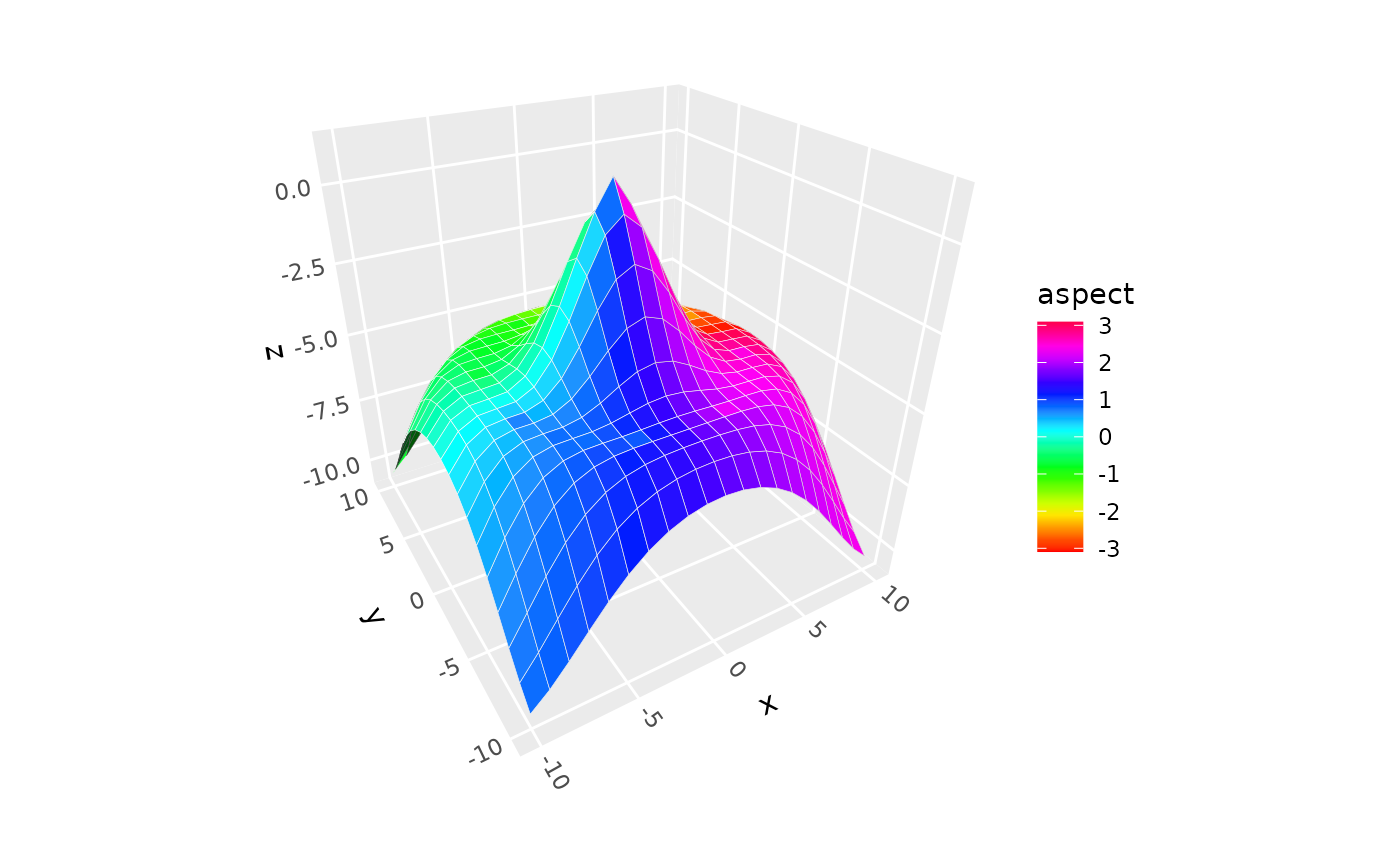
# use after_stat to access computed surface-orientation variables
p + geom_surface_3d(aes(fill = after_stat(aspect))) +
      scale_fill_gradientn(colors = rainbow(20))


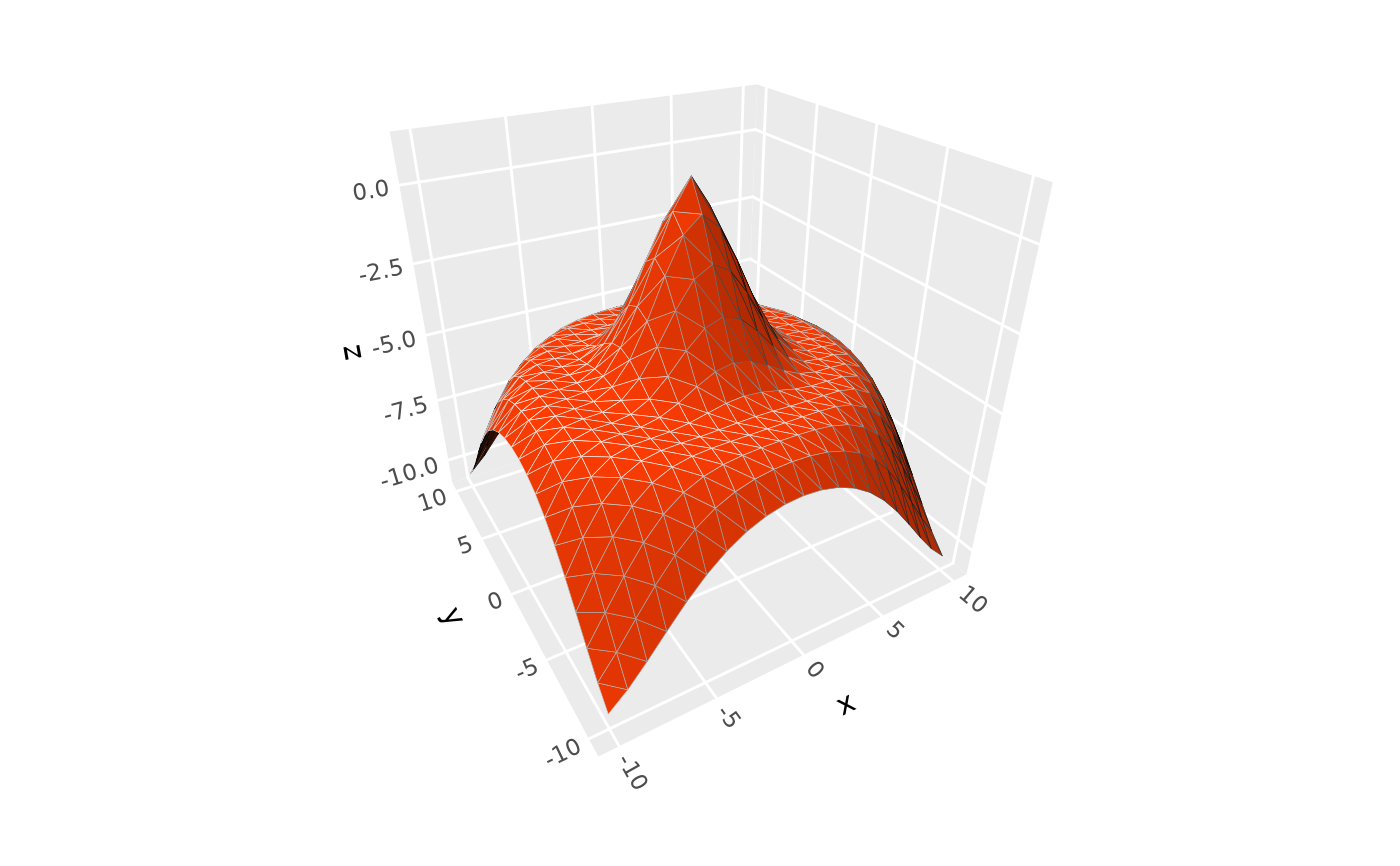
# triangulated surface (can prevent lighting flaws)
p + geom_surface_3d(fill = "#9e2602", color = "black", grid = "tri1")


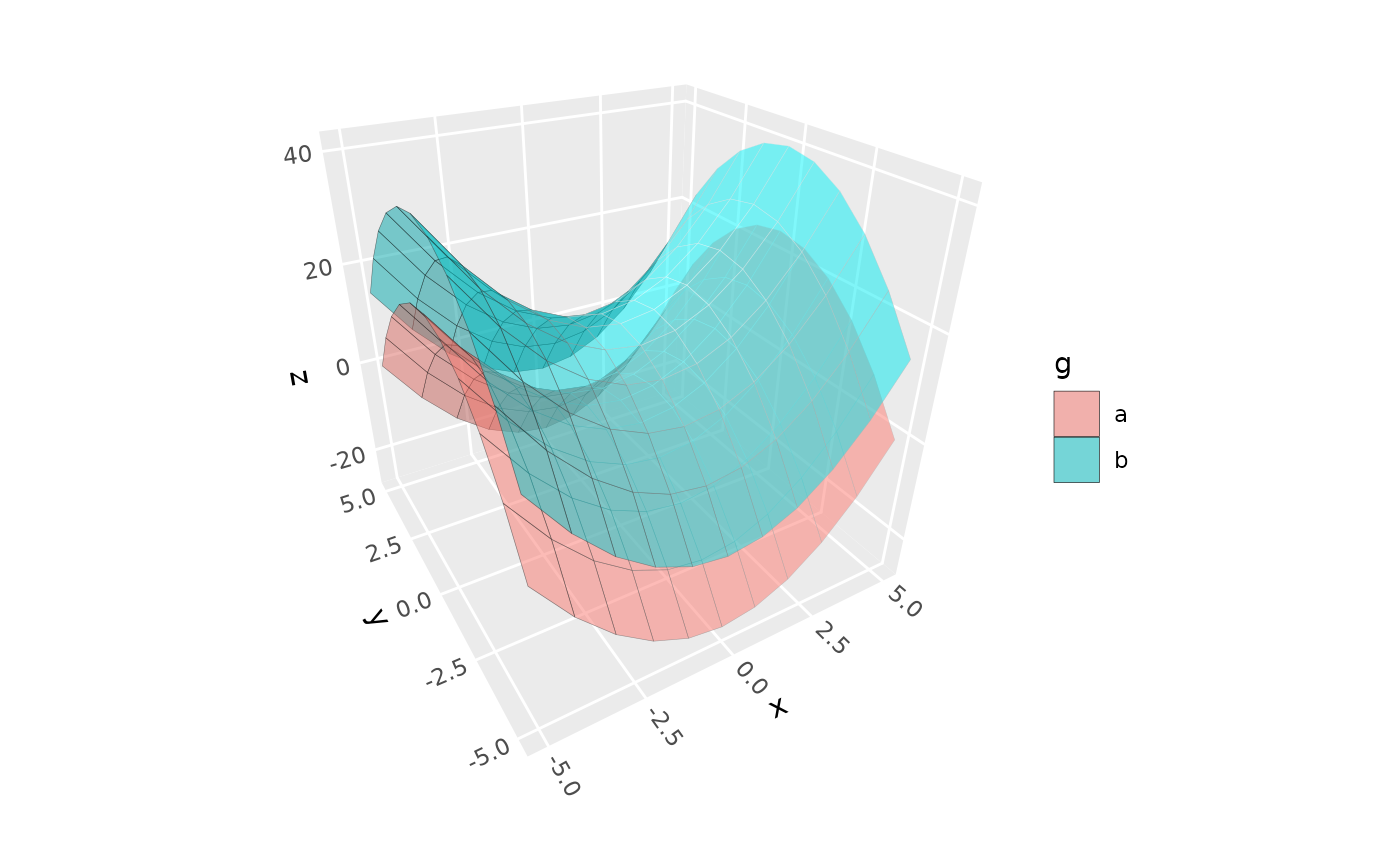
# use `group` to plot data for multiple surfaces
d <- expand.grid(x = -5:5, y = -5:5)
d$z <- d$x^2 - d$y^2
d$g <- "a"
d2 <- d
d2$z <- d$z + 15
d2$g <- "b"
ggplot(rbind(d, d2), aes(x, y, z, group = g, fill = g)) +
  coord_3d() +
  geom_surface_3d(color = "black", alpha = .5, light = NULL)


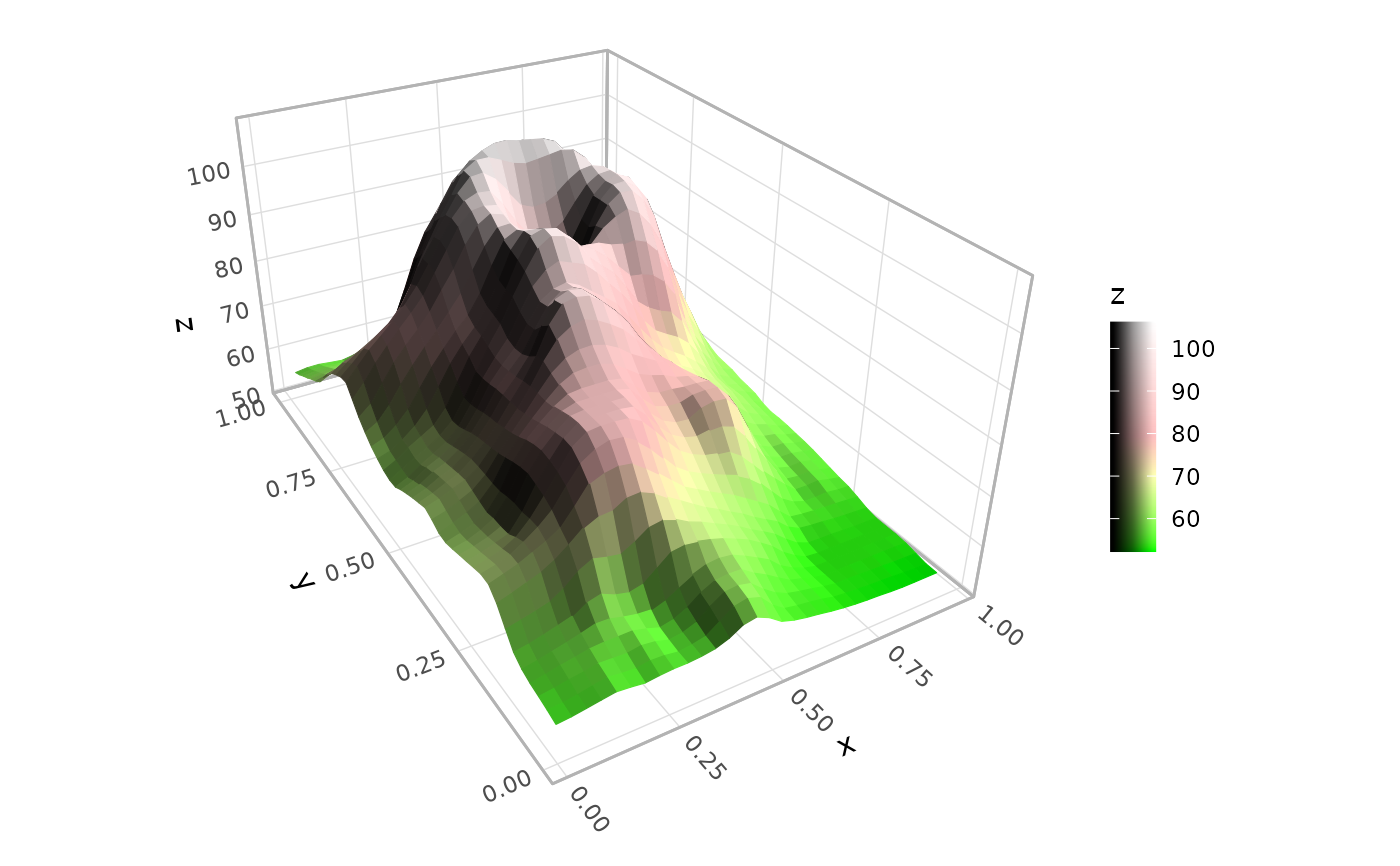
# terrain surface with topographic hillshade and elevational fill
ggplot(mountain, aes(x, y, z, fill = z, color = z)) +
  geom_surface_3d(light = light(direction = c(1, 0, .5),
                           mode = "hsv", contrast = 1.5),
               linewidth = .2) +
  coord_3d(ratio = c(1, 1.5, .75)) +
  theme_light() +
  scale_fill_gradientn(colors = c("darkgreen", "rosybrown4", "gray60")) +
  scale_color_gradientn(colors = c("darkgreen", "rosybrown4", "gray60")) +
  guides(fill = guide_colorbar_3d())