Wind data

Every windscape analysis starts from wind data. This article covers how windscape represents wind, where to get data and how to download it, how to choose the time window for an analysis, how to bring in data from other sources, and how to build, modify, and visualize wind roses.

library(windscape)
library(ggplot2)

states <- map_data("state")
borders <- geom_path(data = states, aes(long, lat, group = group),
                     color = "gray50", linewidth = 0.2, inherit.aes = FALSE)
us <- coord_quickmap(xlim = c(-120, -90), ylim = c(30, 50), expand = FALSE)

How windscape represents wind

windscape uses three classes of wind data, all SpatRasters with some added structure:

A wind_field is the wind at a single moment: two layers, giving the eastward (u) and northward (v) components of the wind vector in each grid cell.
A wind_series is a time series of wind fields: all the u layers, followed by all the v layers, in the same time order.
A wind_rose summarizes a wind series as the average conductance of wind from each cell toward each of its eight neighbors, in eight layers.

All three share some requirements. Data must be on a longitude/latitude grid with approximately square cells, because windscape computes distances and directions between neighboring cells on the earth’s surface. Wind components should be in meters per second, the units that windscape’s travel times, trail lengths, and other outputs assume.

Choosing a data source

windscape can download three gridded wind data sets, all reanalyses: models that combine weather observations with a physical model of the atmosphere to estimate past conditions everywhere, hourly.

Data set	Years	Grid	Heights
ERA5 (ECMWF)	1940 to present	0.25 degrees (about 28 km)	10 m, 100 m
CFSR (NCEP)	1979-2010	about 0.31 degrees (about 35 km)	10 m, pressure levels
CFSv2 (NCEP)	2011 to present	about 0.2 degrees (about 22 km)	10 m, pressure levels

ERA5 is the best default: it is a single, consistent data set with the longest record, on one grid. CFSR is mainly useful for continuity with earlier analyses that used it, including several windscape-based studies. CFSv2 is the operational continuation of CFSR, but splicing the two into one longer record takes care: they are on different grids, so one has to be resampled to match the other before building wind roses, and the change of model in 2011 can introduce a step change in wind speed or direction. For a long continuous record, ERA5 avoids both problems.

The height of the wind data should match where dispersal happens. Winds 10 m above the ground suit most near-surface dispersal, such as seeds and pollen released from vegetation. ERA5’s 100 m winds may better represent transport above forest canopies, or of propagules lofted higher in the atmosphere. CFSR’s and CFSv2’s pressure levels (1000 to 200 hPa, from near the surface to about 12 km) describe winds aloft, relevant for long-distance transport such as insect migration or spores carried high into the atmosphere.

Downloading

ncar_download() downloads data from NCAR’s Geoscience Data Exchange, with no account needed:

files <- ncar_download("era5", level = "10m",
                       xlim = c(-120, -90), ylim = c(30, 50),
                       years = 2011:2020, months = 1:12,
                       time_stride = 3, dir = "~/wind_data")

Data are clipped to the bounding box on the server, so only the region you need is transferred, and each month is saved as a separate file (see ?ncar_download for all options). A few choices deserve thought:

Make the box larger than your study area. Connectivity models lose particles across the edges of the domain, so results near the edges are less reliable.
Consider thinning in time. Winds are strongly autocorrelated from hour to hour, so time_stride = 3 (every third hour) loses little information for building wind roses, while cutting download time and file size about threefold.
Save to a permanent directory. Months already downloaded to dir are skipped, so an interrupted download resumes where it stopped, and extending an analysis to more years only downloads the new ones. The default is a temporary directory.

Downloads can be large: a decade of every-third-hour data for the box above is about 1 GB before compression, so start with a single month to check your settings.

ncar_download() returns the paths of the monthly files. wind_series() combines them into a single wind_series, without reading the data into memory until needed:

series <- wind_series(files)

ncar_land() downloads a land-water layer on the same grid as the wind data, for use with weight_conductance() (see below):

land <- ncar_land("era5", xlim = c(-120, -90), ylim = c(30, 50))

Choosing the time window

windscape’s models describe the average behavior of the wind over the time steps in a wind series, so the choice of time steps is a modeling decision. A few principles:

Use the native time resolution. Averaging winds over time, for example into monthly means, cancels out winds blowing in opposite directions, so averaged winds understate both the speed and the variability of the wind. Use hourly data, or data thinned with time_stride, rather than averages.
Match the record length to the process. For processes that integrate over many years, such as gene flow, use a long record, ideally a decade or more, so that the wind rose reflects typical conditions rather than the quirks of particular years. For dispersal during a particular period, a shorter record may be appropriate.
Match the season and time of day to dispersal. If propagules are only released during part of the year, such as a flowering or fruiting season, or at certain times of day, build the wind rose from those times only.

subset_series() selects time steps by month, hour of day, date range, or index, and wind_times() returns the time of each step. To demonstrate, we’ll use a small example series that ships with the package, covering the western and central US every 6 hours on the 1st and 15th of each month in 2000:

series <- windscape_example("wind_series")
range(wind_times(series))
#> [1] "2000-01-01 00:00:00 UTC" "2000-12-15 18:00:00 UTC"

summer <- subset_series(series, months = 6:8)
winter <- subset_series(series, months = c(12, 1, 2))
c(summer = summer@n_steps, winter = winter@n_steps)
#> summer winter 
#>     24     24

Hours are in UTC. Local solar time is about UTC plus longitude / 15 hours, so for this region, afternoon is roughly 20:00 to 01:00 UTC; for a large region, a given UTC hour falls at different local times in different places.

Pass the selected series to wind_rose() to build a rose from those time steps; this works for long records of downloaded files too (see below). When the selection is known in advance, ncar_download()’s months argument also avoids downloading data you won’t use.

Bringing your own data

Wind data from other sources, such as other reanalyses, regional climate models, or interpolated station data, can be used too. Load the data as a SpatRaster, check that it meets windscape’s requirements, and convert it with wind_series():

x <- terra::rast("my_wind_data.nc")

x <- terra::rotate(x)  # if longitudes run from 0 to 360, convert them to -180 to 180
x <- x / 3.6           # if winds are in km/h, convert them to m/s
series <- wind_series(x, order = "uvuv")

The order argument describes how the layers are arranged: "uuvv" (all u layers, then all v layers), or "uvuv" (alternating). For the time-based features of subset_series() and wind_times(), give the layers times, either in their names (like "u 2000-01-01 06:00:00") or with terra::time(). Data in a projected coordinate system must be reprojected to longitude/latitude with terra::project(), which should be done on the u and v components with care, because projection rotates directions as well as moving cells.

Wind fields

A single time step of a wind series is a wind field. windscape provides ggplot2 layers for drawing them, and ggplot() accepts wind fields directly. Here is the first time step of the example series, with geom_wind_trail() drawing trails that follow the airflow over a map of wind speed:

field <- wind_field(series, step = 1)

ggplot(field, aes(x, y)) +
      geom_raster(aes(fill = speed)) +
      borders +
      geom_wind_trail(color = "white") +
      scale_fill_viridis_c(name = "wind speed\n(m/s)") +
      us + theme_void()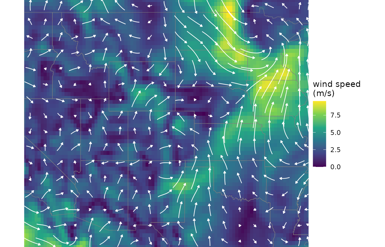

geom_wind_arrow() instead draws an arrow for the average wind in each block of cells, here colored by wind direction with scale_color_bearing(), a circular color scale for compass bearings:

ggplot(field, aes(x, y)) +
      borders +
      geom_wind_arrow(aes(color = after_stat(bearing)), linewidth = 0.5) +
      scale_color_bearing(name = "direction") +
      us + theme_void()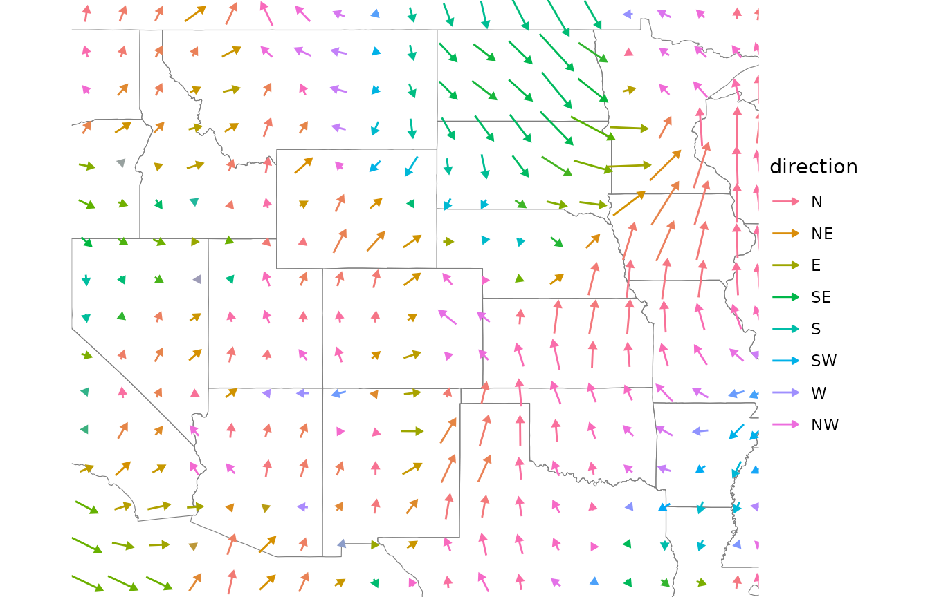

Both layers summarize the field in blocks of cells, with lengths proportional to wind speed by default; see their documentation for options. wind_trails() returns trails as a data frame, which geom_wind_path() draws, and fortify() converts a wind field to a data frame with each cell’s u, v, speed, and bearing, for custom plots.

To summarize a whole series as a single field, mean() returns its time-mean wind: the net drift of the air over the series, which is short where winds blow from many directions, even if they are strong. It can be plotted the same way:

ggplot(mean(series), aes(x, y)) +
      geom_raster(aes(fill = speed)) +
      borders +
      geom_wind_trail(color = "white", hours = 24) +
      scale_fill_viridis_c(name = "mean wind\n(m/s)") +
      us + theme_void()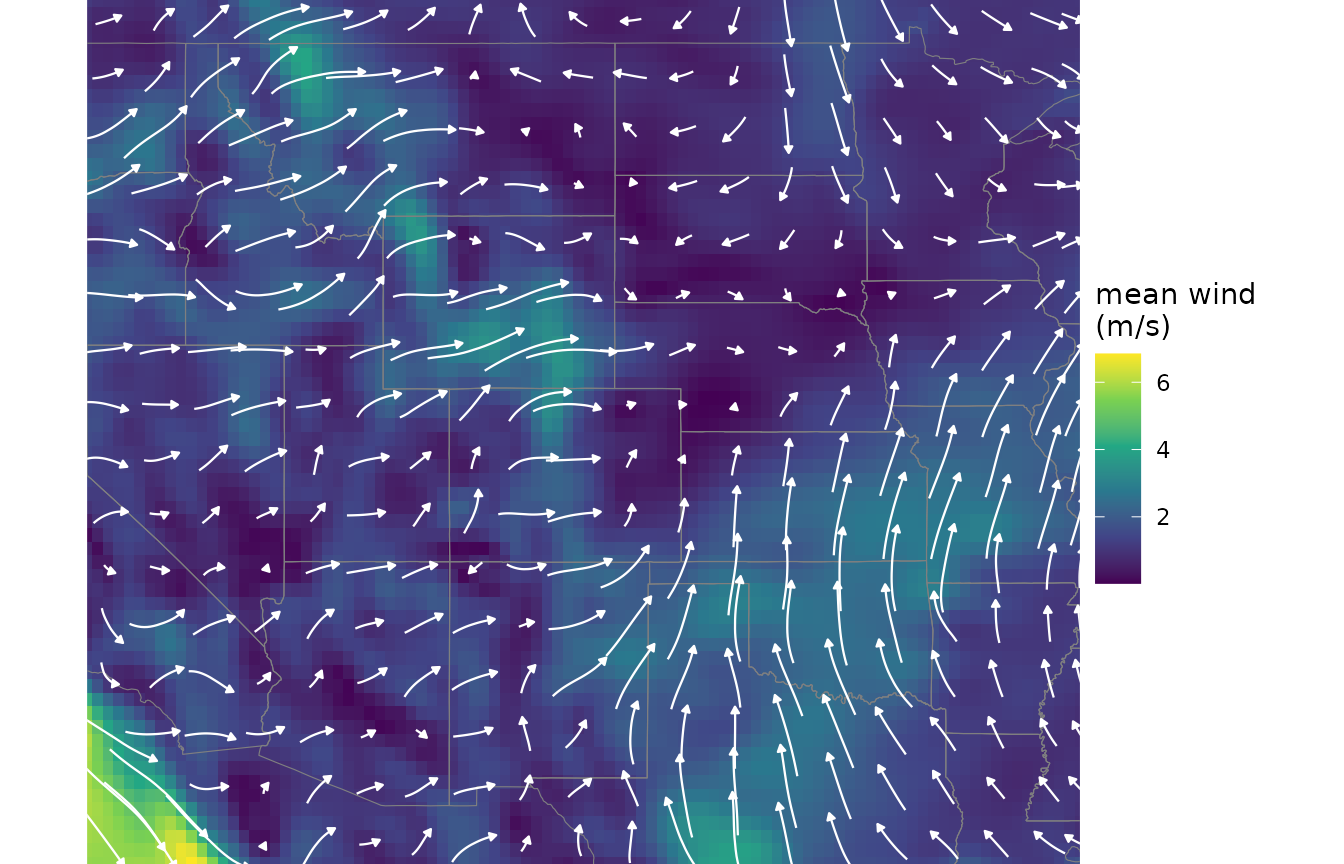

Wind roses

A wind rose summarizes a wind series into a model of the wind regime. For each time step, wind_rose() divides the wind in each cell between the two neighboring cells whose directions bracket the wind direction, in proportion to how closely the wind points toward each, and then averages over all time steps. The result is the mean conductance of wind from each cell toward each of its eight neighbors: the rate at which wind moves material from the cell to that neighbor.

rose <- wind_rose(series)
rose
#> class       : SpatRaster
#> size        : 64, 96, 8  (nrow, ncol, nlyr)
#> resolution  : 0.3157895, 0.3174603  (x, y)
#> extent      : -120.1579, -89.84211, 29.84127, 50.15873  (xmin, xmax, ymin, ymax)
#> coord. ref. : lon/lat WGS 84 (EPSG:4326)
#> source(s)   : memory
#> names       :       SW,        W,       NW,        N,       NE,        E, ...
#> min values  :        0,        0,        0,        0,  0.00034,   0.0003, ...
#> max values  : 0.115176, 0.164829, 0.205505, 0.278183, 0.195127, 0.440725, ...

Choosing `trans`

The trans argument sets how wind speed translates into conductance. With the default, trans = 1, conductance is proportional to wind speed, and conductance has units of 1/hour, so that travel times from least-cost models are in hours. Other choices model dispersal that depends more strongly on wind speed:

A power greater than 1 raises wind speeds to that power, emphasizing strong winds; for example, trans = 3 is proportional to the kinetic energy flux of the wind, which may suit propagules whose release depends on wind strength.
A function of wind speed (in m/s) allows any other relationship, such as a threshold below which no dispersal occurs: trans = function(x) ifelse(x > 6, x, 0).

Units of conductance (and of travel times) are only hours-based with trans = 1; with other choices, they are relative, which is fine for comparing places and directions. The choice can change the wind regime substantially, because strong winds often blow from different directions than average winds. Here are wind roses built with each choice, mapped with geom_wind_rose(), which draws a glyph for each block of cells with rays pointing toward the eight neighbors, colored by the direction of net flow:

roses <- list("1" = rose,
              "3" = wind_rose(series, trans = 3),
              "threshold at 6 m/s" = wind_rose(series, trans = function(x) ifelse(x > 6, x, 0)))
flows <- c("N", "NE", "E", "SE", "S", "SW", "W", "NW")
d <- do.call(rbind, lapply(names(roses), function(k){
      dk <- fortify(roses[[k]])
      dk[flows] <- dk[flows] / mean(dk$speed) # put the roses on a common scale
      data.frame(dk, trans = k)
}))

ggplot(d, aes(x, y)) +
      borders +
      geom_wind_rose(aes(color = trans), fill = NA, res = 8) +
      us + theme_void()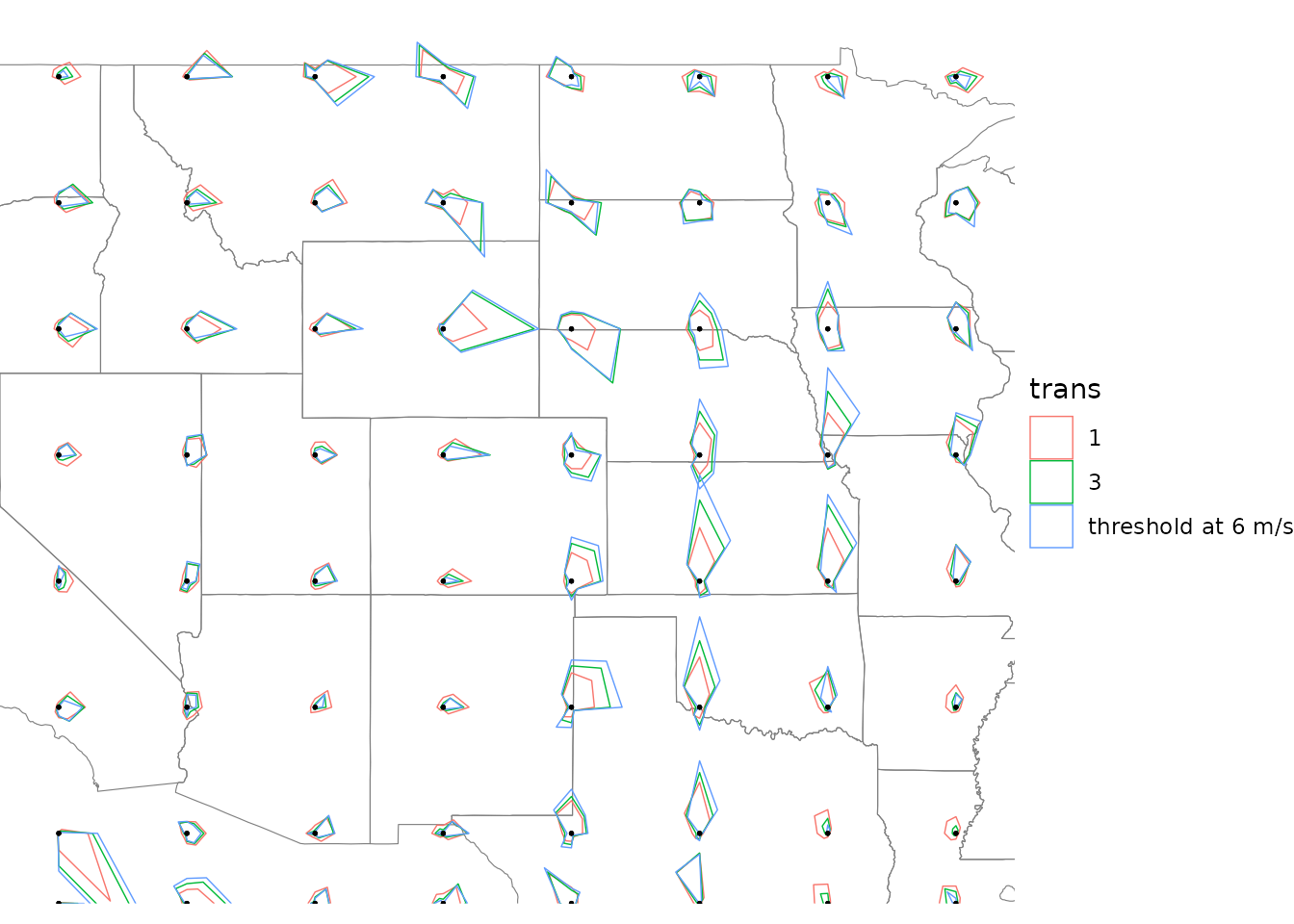

Overlaid glyphs share one scale, and the three choices give conductances in very different units, so each rose’s flows are divided by its mean before plotting. The comparison shows how the pattern of flow changes, not its overall strength: emphasizing strong winds shifts flow toward the directions of the strongest winds and makes it more directional in much of the region.

Seasonal wind roses

Building wind roses from subsets of a wind series shows how the wind regime changes through the year:

d <- rbind(data.frame(fortify(wind_rose(winter)), season = "winter (Dec-Feb)"),
           data.frame(fortify(wind_rose(summer)), season = "summer (Jun-Aug)"))
d$season <- factor(d$season, levels = unique(d$season))

ggplot(d, aes(x, y)) +
      borders +
      geom_wind_rose(aes(color = season), fill = NA, res = 8) +
      us + theme_void()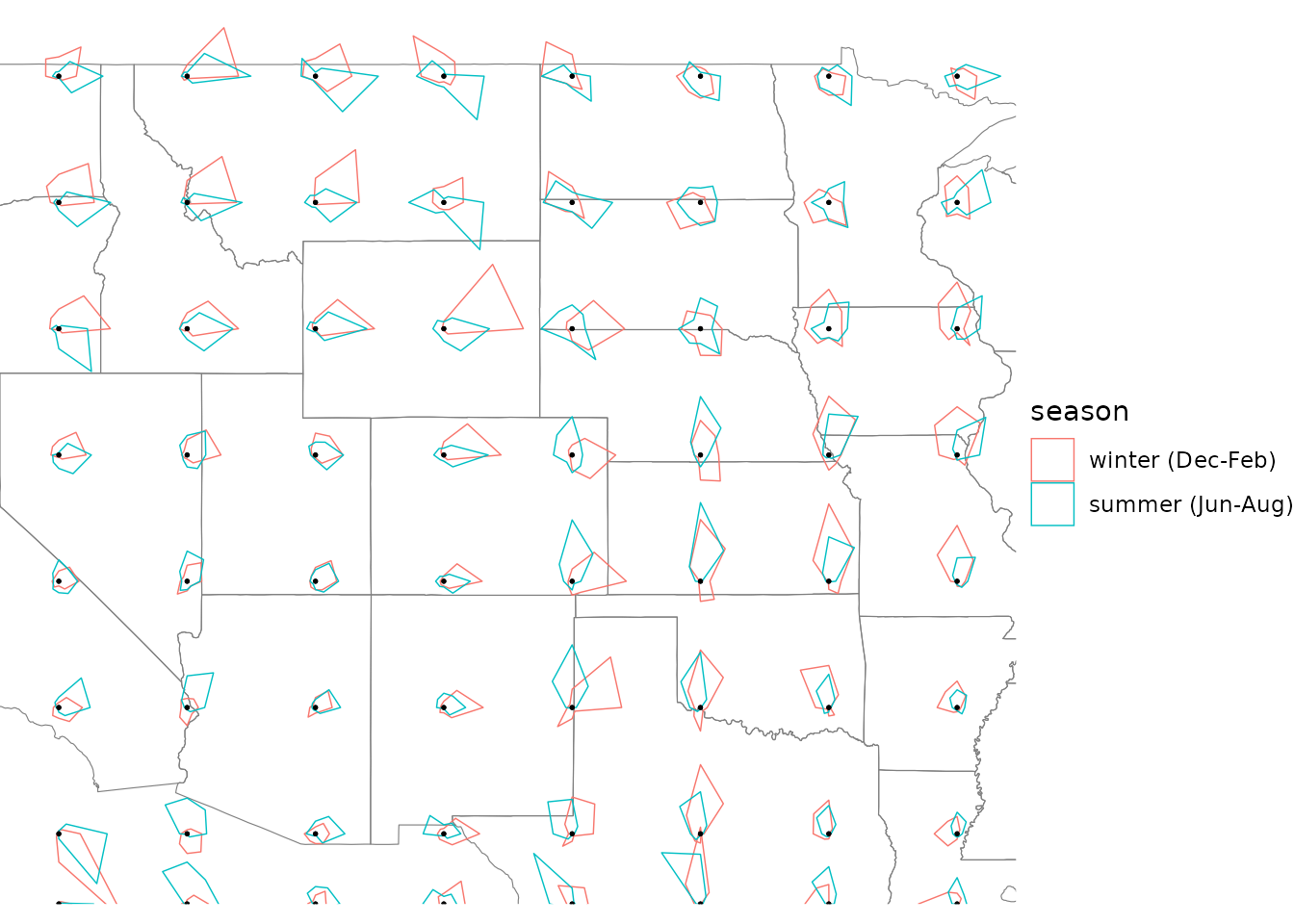

In this sample, winter brings strong southwesterly flow across the interior West. Over the southern plains, winds run north-south in both seasons, but in winter they alternate between northerly and southerly, while in summer they blow mostly from the south. With only 24 time steps per season, these roses are noisy; a real seasonal analysis would use many years of data.

Long records

A wind_series built from downloaded files keeps its data on disk, and wind_rose() processes long series in chunks of time steps, so the whole record never needs to be in memory at once. The result is identical to processing all the time steps together. Selecting time steps with subset_series() also leaves the data on disk, so seasonal or time-of-day roses can be built from long records the same way:

series <- wind_series(files)
rose <- wind_rose(series, trans = 1)

# afternoons during the growing season, across the whole record
rose_gs <- wind_rose(subset_series(series, months = 4:9, hours = c(20:23, 0)))

combine_roses() does the same for roses built separately, for example to add a new year of data to an existing rose. It weights each rose by its number of time steps.

Saving and loading

A wind rose is a SpatRaster and can be saved with terra::writeRaster(). Given a saved rose instead of a wind series, wind_rose() loads it; supply the same trans it was built with, and the number of time steps if you might combine it with other roses later:

terra::writeRaster(rose, "rose.tif")
rose <- wind_rose("rose.tif", trans = 1, n_steps = 29220)

Mapping wind roses

Besides geom_wind_rose(), two tools help map wind roses. net_flow() reduces a rose to a single vector per cell, the net direction and rate of flow, returned as a wind field that can be drawn like any other:

ggplot(net_flow(rose), aes(x, y)) +
      geom_raster(aes(fill = speed)) +
      borders +
      geom_wind_trail(color = "white", hours = 24) +
      scale_fill_viridis_c(name = "net flow\n(m/s)") +
      us + theme_void()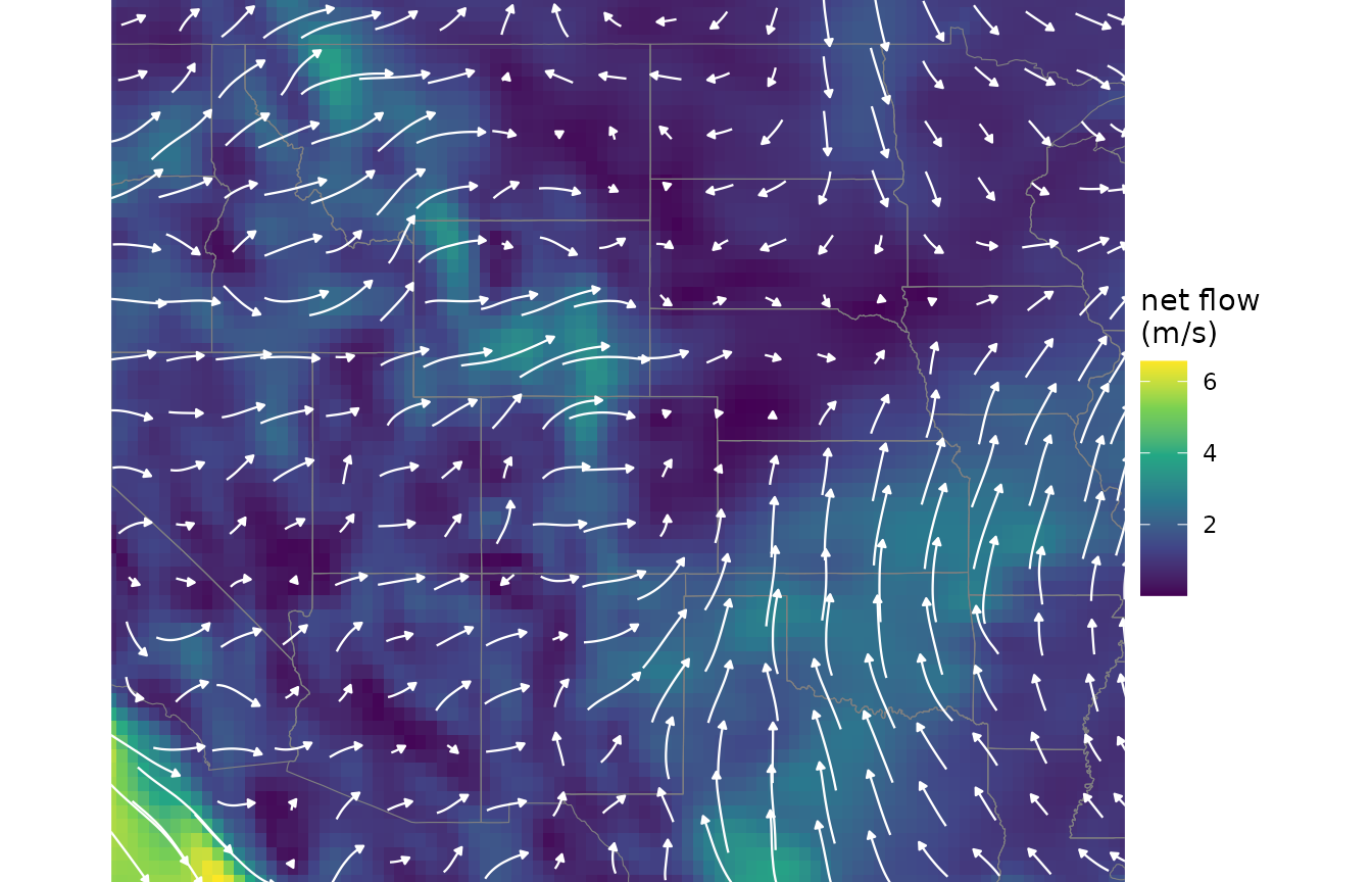

And fortify() converts a rose to a data frame for custom maps. Along with the flow toward each neighbor, it gives each cell’s total flow (speed, the mean wind speed, in km/h), net flow (net), the direction of net flow (bearing), and consistency, the ratio of net to total flow: near 1 where the wind blows predominantly one way, giving strongly directional connectivity, and near 0 where it blows in all directions, spreading material more evenly.

Modifying wind roses

Two functions modify a wind rose before modeling connectivity.

weight_conductance() multiplies conductance by a raster of weights, reducing connectivity through some cells. For example, for terrestrial organisms that can’t establish over water, weighting by the land fraction from ncar_land() reduces connectivity across lakes and oceans (though propagules can still cross them):

land <- ncar_land("era5", xlim = c(-120, -90), ylim = c(30, 50))
rose_land <- weight_conductance(rose, land)

downscale() refines the grid of a wind rose by interpolation. This matters when sites are only a few grid cells apart; see the pairwise connectivity article.