Draw existing wind trails or paths

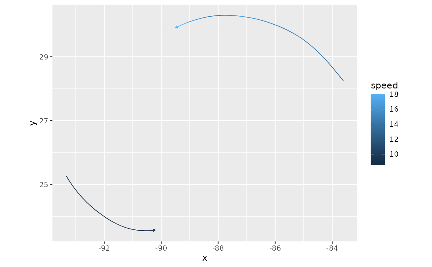
Draws trails or paths you already have as data, such as the output of wind_trails() or least_cost_paths(), as lines with an arrowhead at the downwind end. To compute and draw trails from a wind field in one step, use geom_wind_trail() instead.

Usage

geom_wind_path(
  mapping = NULL,
  data = NULL,
  stat = "identity",
  position = "identity",
  ...,
  arrow = grid::arrow(length = grid::unit(0.1, "cm"), type = "closed"),
  na.rm = FALSE,
  show.legend = NA,
  inherit.aes = TRUE
)

Arguments

mapping

Aesthetic mappings created by ggplot2::aes(). x and y (coordinates, in degrees longitude and latitude) must be mapped, usually in the plot's main call. group and t are mapped automatically to the columns trail and step, as in wind_trails() and least_cost_paths() output: group identifies each trail, and t orders the points along it, from upwind to downwind. Map them in this layer if your columns are named differently.

data

A data frame of trail points. Default is to inherit the plot's data.

stat

The statistical transformation; the default, "identity", draws the data as is.

position

Position adjustment; see ggplot2::layer().

...

Other arguments passed to ggplot2::layer(), such as fixed aesthetics like color = "white" or linewidth = 0.8.

arrow

Arrowhead drawn at the downwind end of each trail, created by grid::arrow(), or NULL for none.

na.rm, show.legend, inherit.aes

See ggplot2::layer().

Value

A ggplot2 layer.

See also

geom_wind_trail() to compute trails from a wind field.

Examples

library(ggplot2)
katrina <- windscape_example("wind_field")
sites <- cbind(c(-92, -86), c(24, 30))
trails <- wind_trails(katrina, sites, hours = 12)

ggplot(trails, aes(x, y)) +
  geom_wind_path(aes(color = speed)) +
  coord_quickmap()