Pairwise connectivity • windscape

Many ecological questions about wind concern a set of sites rather than a single one. Does wind explain gene flow or genetic differentiation among populations? Do pathogens or pests spread along the routes wind favors? Are communities more similar where wind links them strongly? Each of these compares a pairwise matrix of wind connectivity among sites with a pairwise matrix of ecological data.

This article covers estimating pairwise wind connectivity with windscape’s two connectivity models, placing sites on the wind grid, and testing hypotheses about the role of wind with Mantel tests. It uses model settings such as half_life without explaining them in depth; the connectivity models article covers how the models work and how to choose their settings. It ends with a worked example using birch, a landscape genetic data set that ships with the package.

library(windscape)
library(ggplot2)

rose <- windscape_example("wind_rose")

states <- map_data("state")
borders <- geom_path(data = states, aes(long, lat, group = group),
                     color = "gray70", linewidth = 0.15, inherit.aes = FALSE)
us <- coord_quickmap(xlim = c(-120, -90), ylim = c(30, 50), expand = FALSE)

We’ll use twenty random sites across the example rose’s domain:

set.seed(2)
sites <- cbind(lon = runif(20, -114, -96), lat = runif(20, 33, 47))

Least-cost connectivity

pairwise_least_cost() returns a matrix of least-cost wind travel times between every pair of sites, in hours (for a rose built with trans = 1 from winds in m/s):

hours <- pairwise_least_cost(rose, sites)
round(hours[1:5, 1:5])
#>      [,1] [,2] [,3] [,4] [,5]
#> [1,]    0  287  184  807  526
#> [2,] 1063    0  312 1178  330
#> [3,]  879  307    0 1342  467
#> [4,]  605  285  521    0  480
#> [5,] 1221  364  394 1498    0

Element [i, j] is the travel time from site i to site j, so row i describes travel downwind from site i, and column j describes travel upwind to site j. That’s why, unlike least_cost(), this function has no direction argument: the matrix covers both. Because wind is directional, the matrix is asymmetric. Wind takes about 287 hours to carry material from site 1, in southwestern Wyoming, to site 2, in Kansas, but about 1063 hours to carry it back. least_cost_paths() shows the two routes:

routes <- rbind(data.frame(least_cost_paths(rose, sites[1, , drop = FALSE], sites[2, , drop = FALSE]),
                           route = "site 1 to site 2"),
                data.frame(least_cost_paths(rose, sites[2, , drop = FALSE], sites[1, , drop = FALSE]),
                           route = "site 2 to site 1"))
routes$trail <- as.integer(factor(routes$route))

ggplot(routes, aes(x, y)) +
      borders +
      geom_wind_path(aes(color = route), linewidth = 0.8) +
      annotate("point", sites[, 1], sites[, 2], size = 0.8, color = "gray40") +
      annotate("text", sites[1:2, 1], sites[1:2, 2], label = 1:2, vjust = -0.8) +
      scale_color_manual(values = c("darkorange", "dodgerblue")) +
      us + theme_void()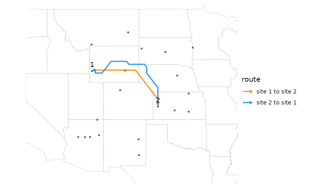

Travel times are a measure of accessibility, small for well-connected pairs. rate = TRUE returns their inverse, a flow rate, which is large for well-connected pairs, matching the orientation of random walk connectivity.

Random walk connectivity

pairwise_random_walk() estimates connectivity with a stream-mode random walk released from each site in turn. By default, element [i, j] is the probability density (per km^2) that a particle released at site i is deposited at site j:

deposition <- pairwise_random_walk(rose, sites, half_life = 48)
signif(deposition[1:5, 1:5], 2)
#>         [,1]    [,2]    [,3]    [,4]    [,5]
#> [1,] 5.1e-05 5.9e-08 1.1e-06 4.3e-16 3.6e-11
#> [2,] 3.9e-18 4.7e-05 2.3e-08 4.1e-19 1.5e-09
#> [3,] 1.1e-15 2.2e-08 5.9e-05 3.7e-21 3.2e-11
#> [4,] 1.7e-11 5.7e-07 3.0e-09 6.2e-05 1.3e-10
#> [5,] 3.6e-19 3.4e-09 4.0e-09 1.8e-22 3.4e-05

A half-life is required under the default value = "deposition", since without it nothing is deposited. value = "residence" instead gives the time particles from site i spend airborne over site j, which works without a half-life. Values are per km^2 of the destination’s grid cell (density = TRUE), because a larger cell catches more of the particles passing over it; on a longitude/latitude grid, cell area shrinks toward the poles, so per-cell values would favor low-latitude destinations.

The diagonal holds each site’s self-connectivity: its own release deposited in its own cell. It’s usually far larger than the other values, and the tests below ignore it.

Deposition spans many orders of magnitude, from relatively large values for close downwind neighbors to vanishingly small ones for distant upwind neighbors, so it’s usually analyzed on a log scale.

Comparing the models

The two models measure different things: the speed of the best route, versus the share of material that arrives along all routes, net of deposition on the way. Plotting one against the other shows how they relate for these sites:

off <- row(hours) != col(hours) # pairs of distinct sites
d <- data.frame(rate = 1 / hours[off], deposition = deposition[off])

ggplot(d, aes(rate, deposition)) +
      geom_point(alpha = 0.5) +
      scale_x_log10() + scale_y_log10() +
      labs(x = "least-cost flow rate (1 / hours)", y = "random walk deposition (per km^2)") +
      theme_minimal()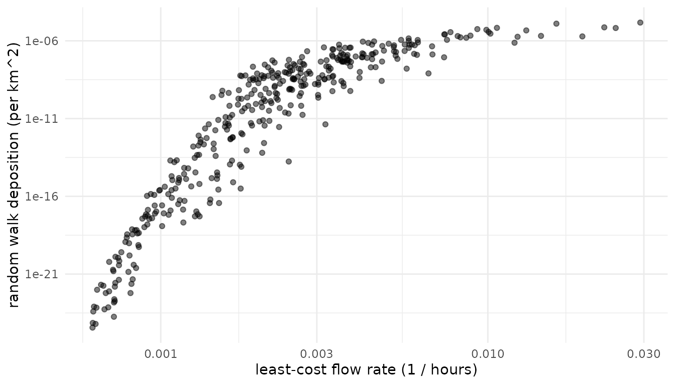


cor(d$rate, d$deposition, method = "spearman")
#> [1] 0.9456101

The models largely agree on which pairs are well connected, but not on how connectivity scales. Among poorly connected pairs, random walk connectivity falls off far faster than flow rate, so it concentrates on near, downwind neighbors. Reaching a distant upwind site requires material to spread against or across the prevailing wind, which becomes exponentially unlikely with distance, while a least-cost route can always wait out the wind. Deposition along the way adds to this, but only modestly: a longer half-life flattens the curve only slightly. The models also diverge where the fastest route is narrow or roundabout, so that little material actually follows it.

Least-cost connectivity suits questions about accessibility, and handles sites that are close together (see below). Random walk connectivity suits questions about how much material is exchanged, such as dispersal or gene flow, especially when deposition along the way matters. Where the choice isn’t clear, testing both is informative.

Placing sites on the grid

Both models work on the wind rose’s grid, but they place sites on it differently, which matters when sites are only a few grid cells apart.

pairwise_least_cost() places sites at their actual locations. It adds each site to the wind graph as a node of its own, linked to the centers of nearby grid cells, and to other nearby sites, by travel times computed exactly for the local wind. It therefore distinguishes sites that are close together, even within the same grid cell. With snap = TRUE, sites are instead moved to the centers of their cells, as in other least-cost tools. Here are three sites, the first two in the same grid cell:

near <- cbind(c(-104.95, -104.75, -104.3), c(40.1, 40.25, 40.15))
terra::cellFromXY(rose, near)
#> [1] 3025 3025 3027

round(pairwise_least_cost(rose, near), 1)
#>      [,1] [,2] [,3]
#> [1,]  0.0 16.0 19.6
#> [2,] 27.8  0.0 17.9
#> [3,] 86.6 71.5  0.0
round(pairwise_least_cost(rose, near, snap = TRUE), 1)
#>      [,1] [,2] [,3]
#> [1,]  0.0  0.0 14.9
#> [2,]  0.0  0.0 14.9
#> [3,] 88.7 88.7  0.0

Snapped, the first two sites are zero hours apart, with identical travel times to and from the third site. Placed at their actual locations, they get distinct travel times, which change smoothly as sites move.

A random walk moves particles from cell to cell, so pairwise_random_walk() treats each site as its grid cell: sites in the same cell get identical rows and columns, and the distances and directions among sites a few cells apart are distorted. check_cell_distance() reports how much the grid distorts the distances among a set of sites:

check_cell_distance(rose, sites)
#> Total point pairs: 190
#> Point pairs in the same grid cell: 0 (0%)
#> Distribution of cell-point distance discrepancies:
#>  0--1%: 90 (47.4%)
#>  1--2.5%: 66 (34.7%)
#>  2.5--5%: 21 (11.1%)
#>  5--10%: 10 (5.26%)
#>  10--25%: 2 (1.05%)
#>  25--Inf%: 1 (0.526%)

None of the twenty sites share a cell, and most discrepancies are a few percent, so this grid suits them. Where many pairs are affected, a finer grid separates nearby sites, from finer wind data or from downscale(), which interpolates a wind rose onto a finer grid. But a random walk’s spread depends on cell size, so a finer grid also changes the model: in one test, downscaling by a factor of 4 narrowed a walk’s spread by 30 to 50 percent. Choose one resolution for an analysis and treat it as part of the model specification; see ?downscale.

Testing hypotheses

Pairwise wind connectivity can be compared with pairwise ecological data to test whether wind shapes ecological patterns. Kling and Ackerly (2021) framed several kinds of hypotheses, each using a different summary of the connectivity matrix:

Flow: is directional wind connectivity related to directional ecological flow, such as gene flow or the spread of a pathogen? Compare the asymmetric matrices directly.
Isolation: are pairs of sites that are poorly connected by wind, in both directions, more different, for example genetically? pairwise_means() averages the two directions into a symmetric matrix of overall connectivity, isolating the effects strength.
Asymmetry: are directional imbalances in wind connectivity related to imbalances in ecological flow? pairwise_ratios() converts a matrix into log ratios of the two directions, log(x[i, j] / x[j, i]), isolating the effects of direction.

pairwise_ratios() also accepts a vector of site attributes, returning the log ratio of each pair’s values. This supports site-level hypotheses such as whether sites that receive more wind than they send, being downwind of the others, have higher genetic diversity (see the worked example below).

Mantel tests

The values in a pairwise matrix aren’t independent, since each site contributes to many pairs, so ordinary correlation tests overstate significance. mantel_test() assesses significance by permuting sites, rearranging the rows and columns of one matrix together. Unlike most Mantel implementations, it handles asymmetric matrices and partial tests with several control matrices (z), such as geographic distance or environmental difference. Diagonals are ignored.

To demonstrate, we’ll simulate gene flow that partly reflects wind connectivity, and genetic differentiation that is low where gene flow is high:

set.seed(1)
n <- nrow(sites)
log_flow <- log(deposition) + rnorm(n^2, sd = 8) # wind signal plus noise
gene_flow <- exp(log_flow)
gene_diff <- pairwise_means(matrix(rnorm(n^2, sd = 4), n)) - pairwise_means(log_flow)

distance <- point_distance(sites) # km

Now we test each hypothesis, controlling for geographic distance in the flow and isolation tests, since nearby sites tend to be both well connected by wind and ecologically similar. (Distance control is unneeded for the asymmetry test, since pairwise_ratios() generates reciprocally symmetrical matrices that, by construction, are uncorrelated with symmetric covariates like distance.)

tests <- list(
      flow = mantel_test(log(deposition), log(gene_flow), z = list(distance)),
      isolation = mantel_test(log(pairwise_means(hours)), gene_diff, z = list(distance)),
      asymmetry = mantel_test(pairwise_ratios(deposition), pairwise_ratios(gene_flow)))

sapply(tests, function(x) round(c(stat = x$stat, p.value = x$p.value), 3))
#>          flow isolation asymmetry
#> stat    0.792     0.429     0.858
#> p.value 0.000     0.000     0.000

All three relationships are detected, as they should be for data simulated this way. A few points matter for real analyses:

Orientation. Travel times are small for well-connected pairs, and deposition and flow rates are large. The isolation test above expects a positive correlation, because pairs that take longer to reach each other should be more differentiated; with deposition it would be negative. Using rate = TRUE for least-cost matrices puts both models in the same orientation.
Transformations. Connectivity values are strongly skewed, and deposition spans many orders of magnitude, so log transformations usually make relationships closer to linear. Mantel tests use Pearson correlation by default; method = "spearman" tests rank correlation instead.
Power. Mantel tests have limited power with few sites. The number of permutations (nperm, default 999) sets the resolution of p-values: a p-value of 0, as above, means no permutation matched the observed correlation, and is better reported as p < 0.001.
Model settings. Results can depend on the model and its settings, such as half_life and trans. Choose these from the biology of the system where possible, and report how sensitive results are to them, rather than searching for the settings that fit best.

Worked example: silver birch

The birch data set holds landscape genetic data for silver birch (Betula pendula) from 29 populations across Eurasia (Tsuda et al. 2017): site coordinates, allelic richness at each site (div), pairwise relative gene flow (mig), and pairwise genetic differentiation (fst).

str(birch, max.level = 1, give.attr = FALSE)
#> List of 4
#>  $ sites: num [1:29, 1:2] -4.84 -3 -0.92 2.37 22.38 ...
#>  $ div  : num [1:29] 2.79 2.56 2.51 2.17 2.95 2.72 2.5 2.31 2.43 2.5 ...
#>  $ mig  : num [1:29, 1:29] NA 0.3639 0.177 0.0924 0.1306 ...
#>  $ fst  : num [1:29, 1:29] NA 0.0422 0.041 0.1205 0.03 ...

The sites span Europe and Siberia, outside the example wind data, so the code below starts by downloading wind for the region. It isn’t run here, since the download is large.

files <- download_wind_data("era5", xlim = c(-15, 100), ylim = c(35, 72),
                       years = 2011:2020, hours = c(0, 6, 12, 18), dir = "~/wind_data")
rose <- wind_rose(wind_series(files), trans = 1)

With the rose in hand, the analysis follows the steps above. Here we use least-cost flow rates, so that every matrix is oriented with large values meaning strong connectivity:

sites <- birch$sites
wind <- pairwise_least_cost(rose, sites, rate = TRUE)
distance <- point_distance(sites)

tests <- list(
      # does gene flow follow wind?
      flow = mantel_test(log(wind), log(birch$mig), z = list(distance)),
      # are populations poorly connected by wind more differentiated?
      isolation = mantel_test(log(pairwise_means(wind)), birch$fst, z = list(distance)),
      # is gene flow stronger in the direction wind favors?
      asymmetry = mantel_test(pairwise_ratios(wind), pairwise_ratios(birch$mig)),
      # are populations downwind of others more diverse?
      diversity = mantel_test(pairwise_ratios(wind), pairwise_ratios(birch$div)))

sapply(tests, function(x) round(c(stat = x$stat, p.value = x$p.value), 3))

The flow and asymmetry tests expect positive correlations, and the isolation test a negative one. For the diversity test, pairwise_ratios(wind)[i, j] is large when wind favors flow from site i to site j, putting j downwind, so if downwind sites are more diverse, pairwise_ratios(birch$div)[i, j], the log of div[i] / div[j], should be small: the test expects a negative correlation. Swapping in pairwise_random_walk() tests the same hypotheses with random walk connectivity.

References

Kling, M. M., and D. D. Ackerly. 2021. Global wind patterns shape genetic differentiation, asymmetric gene flow, and genetic diversity in trees. Proceedings of the National Academy of Sciences 118: e2017317118.
Tsuda, Y., V. Semerikov, F. Sebastiani, G. G. Vendramin, and M. Lascoux. 2017. Multispecies genetic structure and hybridization in the Betula genus across Eurasia. Molecular Ecology 26: 589-605.