This vignette covers topics related to alpha diversity and endemism, including calculation of basic diversity metrics as well as statistical significance testing using null randomization.
To get started, let’s load the phylospatial library, as
well as tmap for visualization. Note that the functions
covered here all require a phylospatial object as input;
see vignette("phylospatial-data") for details on
constructing data sets. We’ll use the moss() example data
here.
library(phylospatial); library(tmap)
ps <- moss()
Diversity measures
The ps_diversity() function calculates the following
alpha diversity measures. While there are a wide variety of
phylogentically-informed diversity metrics in the literature, the
phylospatial package focuses primarily on “node-based”
diversity metrics like Faith’s PD that give equal treatment to
clades/branches at all levels. Phylogenetic diversity metrics can be
categorized as addressing richness, divergence, and regularity (Tucker
et al. 2017), as listed below. Note that an alternative approach to
assessing divergence is through null model analysis of richness metrics,
discussed later in this vignette.
Richness metrics:
- PD: Phylogenetic diversity, i.e. total length of all branch segments present in a location
- PE: Phylogenetic endemism, i.e. endemism-weighted PD
- ShPD: Shannon’s pylogenetic diversity, a.k.a “phylogenetic entropy”
- ShPE: Shannon’s pylogenetic diversity, weighted by endemism
- SiPD: Simpson’s phylogenetic diversity
- SiPE: Simpson’s phylogenetic diversity, weighted by endemism
- TR: Terminal richness, i.e. richness of terminal taxa (in many cases these are species). For binary data this is the total number of terminals in a site, while for quantitative data it is the sum of probability or abundance values.
- TE: Terminal endemism, i.e. total endemism-weighted diversity of terminal taxa (a.k.a. “weighted endemism”)
- CR: Clade richness, i.e. richness of taxa at all levels (equivalent to PD on a cladogram)
- CE: Clade endemism, i.e. total endemism-weighted diversity of taxa at all levels (equivalent to PE on a cladrogram)
Divergence metrics:
- RPD: Relative phylogenetic diversity, i.e. mean branch segment length of residents (equivalent to PD / CR)
- RPE: Relative phylogenetic endemism, i.e. mean endemism-weighted branch length (equivalent to PE / CE)
- MPDT: Mean pairwise distance between terminals, i.e. the classic MPD measure
- MPDN: Mean pairwise distance between nodes, a node-based version of MPD that calculates the average branch length separating all pairs of collateral (non-lineal) nodes including terminals and internal nodes, giving more representation to deeper branches
Regularity metrics:
- VPDT: Variance in pairwise distances between terminals
- VPDN: Variance in pairwise distances between collateral nodes
All measures use quantitative community data if provided. “Endemism”
is the inverse of the total occurrence mass (the sum of presence,
probability, or abundance values) across all sites in the analysis. See
?ps_diversity for equations giving the derivation of each
metric.
Let’s compute some diversity metrics for our phylospatial data set.
Since our data is raster-based, by default the function will return a
SpatRaster with a layer for each measure. Here we’ll make
plots of PD and PE:
div <- ps_diversity(ps, metric = c("PD", "PE"))
tm_shape(div$PD) +
      tm_raster(col.scale = tm_scale_continuous(values = "inferno")) +
      tm_layout(legend.outside = TRUE)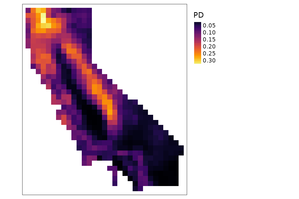
tm_shape(div$PE) +
      tm_raster(col.scale = tm_scale_continuous(values = "inferno")) +
      tm_layout(legend.outside = TRUE)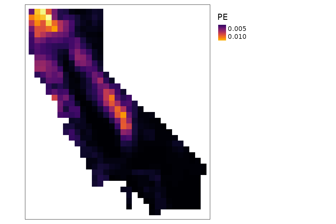
Null model randomization
We can also use randomization to calculate the statistical
significance of these diversity metrics under a null model, using the
ps_rand() function. phylospatial supports a
wide range of randomization schemes via the vegan and
nullcat libraries. Here let’s run our randomization using
quantize, a stratified randomization scheme designed for
use with continuous occurrence data, in combination with a null model
algorithm called "curvecat", which is a categorical version
of the “curveball” algorithm that holds marginal row and column
multisets fixed.
This is a “sequential” (Markov chain) randomization algorithm and
thus requires sufficient iterations to reach stationarity, so before
running our randomizations, we need to decide how many iterations to run
each randomization for. To get an estimate of how many iterations are
necessary for convergence based on our particular data and algorithm
choice, we can call ps_suggest_n_iter() (importantly, using
all the same parameters we plan to use for ps_rand()):
set.seed(123)
iters <- ps_suggest_n_iter(ps, fun = "quantize", method = "curvecat",
                           n_iter = 3e5, plot = TRUE)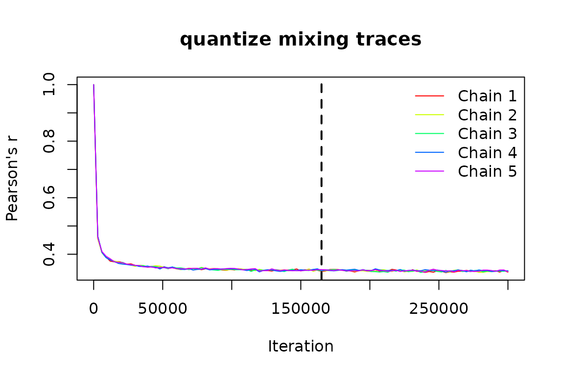
This suggests we need around 200,000 iterations for our matrix to mix
sufficiently, so we’ll pass that value to ps_rand(). Let’s
generate a null distribution of n_rand = 1000 randomized
matrices against which to compare our actual data; we can use
parallelization to speed things up by setting n_cores. Then
we’ll plot the results for PE. This is a quantile value that gives the
proportion of randomizations in which observed PE was greater than
randomized PE in a given grid cell. (If you wanted to identify
“statistically significant” grid cells in a one-tailed test with alpha =
0.05, these would be cells with values greater than 0.95.)
rand <- ps_rand(ps, n_rand = 1000, progress = FALSE,
                metric = c("PD", "PE", "CE", "RPE"),
                fun = "quantize", method = "curvecat",
                n_iter = iters, n_cores = 8)
tm_shape(rand$qPE) +
      tm_raster(col.scale = tm_scale_continuous(values = "inferno")) +
      tm_layout(legend.outside = TRUE)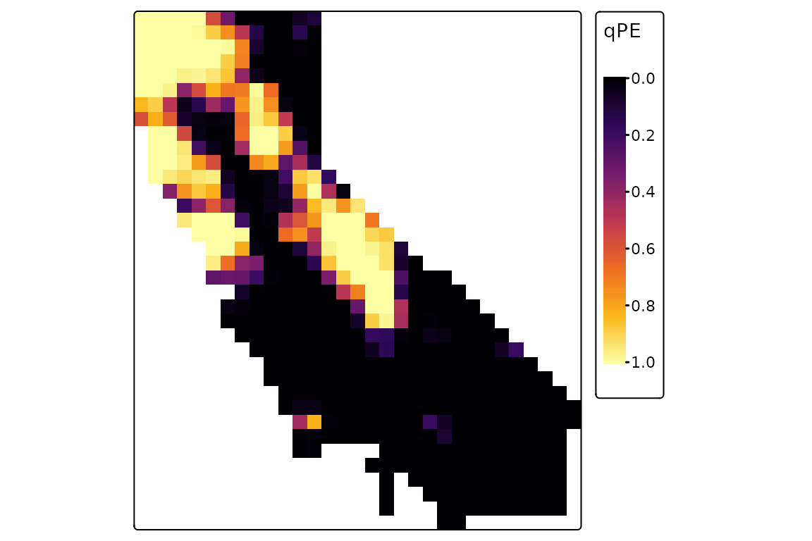
There are numerous alternative options for randomization algorithms,
a choice that will depend on the type of occurrence data you have
(probability, binary, or abundance) and on which attributes of the
terminal community matrix (fill, row and column sums, etc.) you want to
hold fixed. In addition to the "quantize" function used
above, these include “nullcat" randomizations for binary
data, a basic "tip_shuffle" randomization (the default
algorithm), a range of algorithms defined in the vegan
package "nullmodel" function, and an option to supply a
custom randomization function. As a second example, here’s a
randomization with an abundance data set, using the
"abuswap_c" algorithm provided by
vegan::nullmodel (note that since
ps_suggest_n_iter() doesn’t work with vegan,
we need to set n_iter arbitrarily):
ps2 <- ps_simulate(data_type = "abundance")
rand2 <- ps_rand(ps2, fun = "nullmodel", method = "abuswap_c", metric = "PD",
                 n_iter = 1e6, n_rand = 999)
Spatially constrained randomization
Standard null models treat all sites as exchangeable, meaning that species can be shuffled between any pair of sites regardless of how far apart they are. This may not be ecologically realistic: species are more likely to co-occur at nearby sites than distant ones. Spatially constrained null models address this by weighting the randomization so that exchanges occur more frequently between nearby sites. Weights can be continuous or binary and can reflect geographic proximity, environmental similarity, presence in discrete geographic regions, or other spatial properties.
Weighting is available for fun = "quantize" (for
quantitative data) and fun = "nullcat" (for binary data),
but not for fun = "vegan" methods. For eligible methods,
the wt_row argument to ps_rand() accepts a
square weight matrix controlling which pairs of sites are likely to
exchange species during randomization. A natural choice is a
distance-decay function of geographic distance, which can be computed
using ps_geodist(); the choice of decay function and
bandwidth will affect the strength of the spatial constraint, and should
be based on the spatial scale of ecological processes in the study
system. The code below demonstrates weight matrix construction for a few
common shapes of decay function (Gaussian, exponential, threshold), and
also for a scheme involving isolated subregions (e.g. islands) that
never exchange species. Note that adding weights generally increases the
value of n_iter needed for convergence.
# Weight matrices for several alternative distance functions
geo <- as.matrix(ps_geodist(ps_bin)) / 1000 # distance in km
W <- dnorm(geo, sd = 100) # Gaussian decay w0th 100 km SD
W <- exp(-geo / median(geo)) # exponential kernel
W <- (geo < 200) + 0 #  hard distance threshold

# Weights matrix for discrete isolated regions
island <- sample(1:5, nrow(ps$comm), replace = T)
W <- (as.matrix(dist(island)) == 0) + 0

# Spatially constrained randomization
iters <- ps_suggest_n_iter(ps_bin, fun = "nullcat", method = "curvecat", n_iter = 3e5)
rand_spatial <- ps_rand(ps_bin, fun = "nullcat", method = "curvecat", n_iter = iters,
                        n_rand = 1000, metric = c("PD", "PE"),
                        wt_row = W)
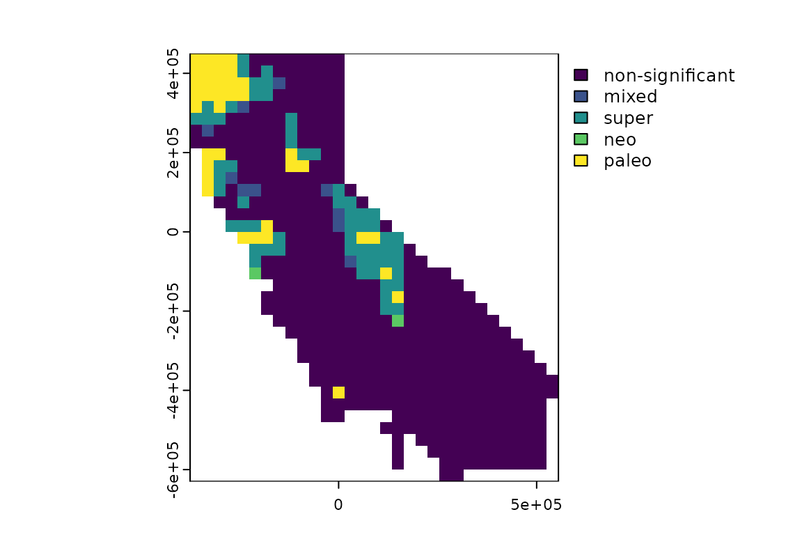
CANAPE
A lot can be done with randomization results like the ones we
generated above. One thing you can do is use them to classify
significant endemism hotspots in a “categorical analysis of neo- and
paleo-endemism” (CANAPE, Mishler et al. 2014). The
function ps_canape() uses significance values for PE, RPE,
and CE, which are returned by ps_rand(), to categorize
sites into five endemism cateogories. Here’s an example with the moss
data; note that depending on the randomization, only a subset of the
five categories may occur in the result here:
