3D surface from 2D density estimate

A 3D version of ggplot2::geom_density_2d(). Creates surfaces from 2D point data using kernel density estimation. The density values become the z-coordinates of the surface, allowing visualization of data concentration as peaks and valleys in 3D space.

Usage

geom_density_3d(
  mapping = NULL,
  data = NULL,
  stat = StatDensity3D,
  position = "identity",
  ...,
  n = NULL,
  grid = NULL,
  direction = NULL,
  trim = NULL,
  h = NULL,
  adjust = 1,
  pad = 0.1,
  min_ndensity = 0,
  light = NULL,
  cull_backfaces = FALSE,
  sort_method = NULL,
  force_convex = TRUE,
  scale_depth = TRUE,
  na.rm = FALSE,
  show.legend = NA,
  inherit.aes = TRUE
)

stat_density_3d(
  mapping = NULL,
  data = NULL,
  geom = GeomPolygon3D,
  position = "identity",
  ...,
  n = NULL,
  grid = NULL,
  direction = NULL,
  trim = NULL,
  h = NULL,
  adjust = 1,
  pad = 0.1,
  min_ndensity = 0,
  light = NULL,
  cull_backfaces = FALSE,
  sort_method = NULL,
  force_convex = TRUE,
  scale_depth = TRUE,
  na.rm = FALSE,
  show.legend = NA,
  inherit.aes = TRUE
)

Arguments

mapping: Set of aesthetic mappings created by aes(). This stat requires x and y aesthetics. By default, fill is mapped to after_stat(density) and z is mapped to after_stat(density).
data: The data to be displayed in this layer. Must contain x and y columns with point coordinates.
stat: The statistical transformation to use on the data. Defaults to StatDensity3D.
position: Position adjustment, defaults to "identity". To collapse the result onto one 2D surface, use position_on_face().
...: Other arguments passed on to the the layer function (typically GeomPolygon3D), such as aesthetics like colour, fill, linewidth, etc.
grid, n, direction, trim: Parameters determining the geometry, resolution, and orientation of the surface grid. See grid_generation for details.
h: Bandwidth vector. If NULL (default), uses automatic bandwidth selection via MASS::bandwidth.nrd(). Can be a single number (used for both dimensions) or a vector of length 2 for different bandwidths in x and y directions.
adjust: Multiplicative bandwidth adjustment factor. Values greater than 1 produce smoother surfaces; values less than 1 produce more detailed surfaces. Default is 1.
pad: Proportional range expansion factor. The computed density grid extends this proportion of the raw data range beyond each data limit. Default is 0.1.
min_ndensity: Lower cutoff for normalized density (computed variable ndensity described below), below which to filter out results. This is particularly useful for removing low-density corners of rectangular density grids when density surfaces are shown for multiple groups, as in the example below. Default is 0 (no filtering).
light: A lighting specification object created by light() (see that function for details), or NULL to disable shading. Specify plot-level lighting in coord_3d() and layer-specific lighting in geom_*3d() functions.
cull_backfaces, sort_method, force_convex, scale_depth: Advanced polygon rendering parameters. See polygon_rendering for details.
na.rm: If FALSE, missing values are removed.
show.legend: Logical indicating whether this layer should be included in legends.
inherit.aes: If FALSE, overrides the default aesthetics.
geom: The geometric object used to display the data. Defaults to GeomPolygon3D.

Value

A Layer object that can be added to a ggplot.

Aesthetics

stat_density_3d() requires the following aesthetics from input data:

x: X coordinate of data points
y: Y coordinate of data points

And optionally understands:

group: Grouping variable for computing separate density surfaces
Additional aesthetics are passed through for surface styling

Computed variables specific to StatDensity3D

density: The kernel density estimate at each grid point
ndensity: Density estimate scaled to maximum of 1 within each group
count: Density estimate × number of observations in group (expected count)
n: Number of observations in each group

Grouping

When aesthetics like colour or fill are mapped to categorical variables, stat_density_3d() computes separate density surfaces for each group, just like stat_density_2d(). Each group gets its own density calculation with proper count and n values.

Computed variables

The following computed variables are available via after_stat():

x, y, z: Grid coordinates and function values
normal_x, normal_y, normal_z: Surface normal components
slope: Gradient magnitude from surface calculations
aspect: Direction of steepest slope from surface calculations
dzdx, dzdy: Partial derivatives from surface calculation

Examples

library(ggplot2)

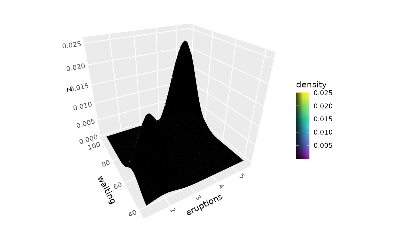
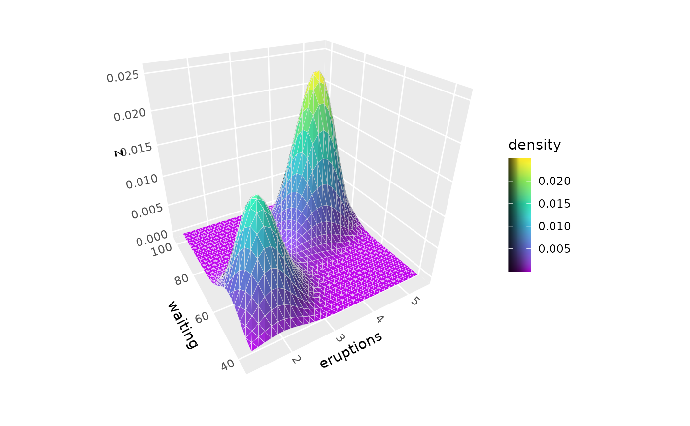
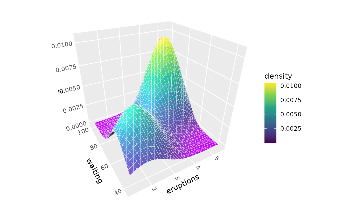
# Basic density surface from scattered points
p <- ggplot(faithful, aes(eruptions, waiting)) +
  coord_3d() +
  scale_fill_viridis_c()

p + geom_density_3d() + guides(fill = guide_colorbar_3d())


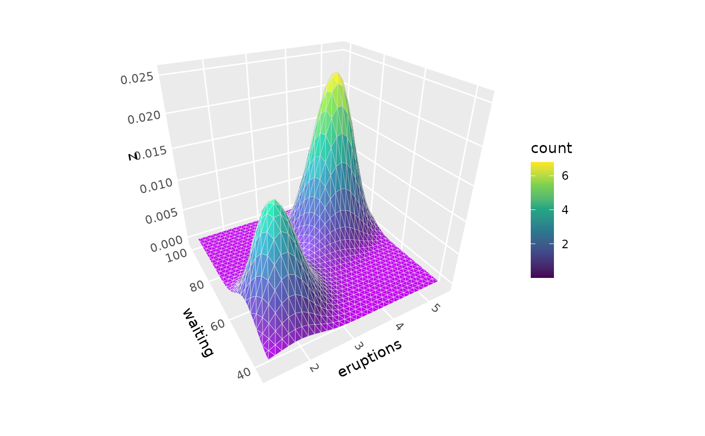
# Color by alternative density values
p + geom_density_3d(aes(fill = after_stat(count)))


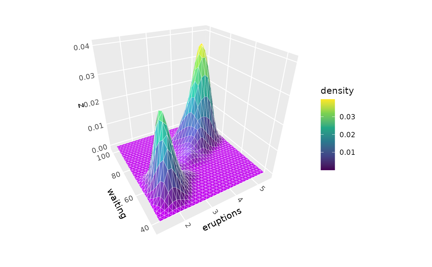
# Adjust bandwidth for smoother or more detailed surfaces
p + geom_density_3d(adjust = 0.5, color = "white")  # More detail

p + geom_density_3d(adjust = 2, color = "white")   # Smoother


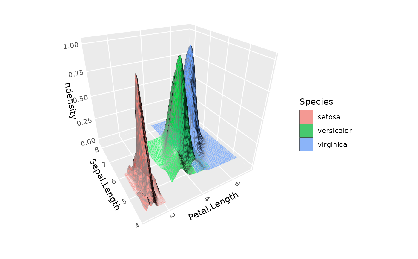
# Multiple density surfaces by group,
# using normalized density to equalize peak heights
ggplot(iris, aes(Petal.Length, Sepal.Length, fill = Species)) +
  geom_density_3d(aes(z = after_stat(ndensity), group = Species),
                  color = "black", alpha = .7, light = NULL) +
  coord_3d()


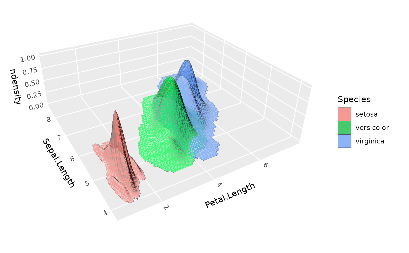
# Same, but with extra padding to remove edge effects and
# with density filtering to remove rectangular artifacts
ggplot(iris, aes(Petal.Length, Sepal.Length, fill = Species)) +
  geom_density_3d(aes(z = after_stat(ndensity)),
                  pad = .3, min_ndensity = .001,
                  color = "black", alpha = .7, light = NULL) +
  coord_3d(ratio = c(3, 3, 1))


# Specify alternative grid geometry and light model
p + geom_density_3d(grid = "hex", n = 30, direction = "y",
                    light = light("direct"),
                    color = "white", linewidth = .1) +
  guides(fill = guide_colorbar_3d())