Computes 1D kernel density estimates for each group and arranges them as
ridgeline polygons in 3D space. Similar to ggridges::geom_density_ridges(),
but rendered as 3D surfaces using geom_ridgeline_3d().
Usage
stat_distributions_3d(
  mapping = NULL,
  data = NULL,
  geom = "ridgeline_3d",
  position = "identity",
  ...,
  direction = NULL,
  bw = "nrd0",
  adjust = 1,
  kernel = "gaussian",
  n = 512,
  trim = FALSE,
  bounds = c(-Inf, Inf),
  rel_min_height = 0,
  joint_bandwidth = FALSE,
  base = 0,
  light = NULL,
  cull_backfaces = FALSE,
  sort_method = NULL,
  scale_depth = TRUE,
  force_convex = FALSE,
  na.rm = FALSE,
  show.legend = NA,
  inherit.aes = TRUE
)

geom_distributions_3d(
  mapping = NULL,
  data = NULL,
  stat = "distributions_3d",
  position = "identity",
  ...,
  direction = NULL,
  bw = "nrd0",
  adjust = 1,
  kernel = "gaussian",
  n = 512,
  trim = FALSE,
  bounds = c(-Inf, Inf),
  rel_min_height = 0,
  joint_bandwidth = FALSE,
  base = 0,
  light = NULL,
  cull_backfaces = FALSE,
  sort_method = NULL,
  scale_depth = TRUE,
  force_convex = FALSE,
  na.rm = FALSE,
  show.legend = NA,
  inherit.aes = TRUE
)
Arguments
- mapping
Set of aesthetic mappings created by
aes(). This stat requiresxandyaesthetics. One of these serves as the grouping/position variable (determined bydirection), and the other provides values for density estimation.- data
The data to be displayed in this layer.
- geom
The geometric object to use to display the data. Defaults to
geom_ridgeline_3d().- position
Position adjustment, defaults to "identity". To collapse the result onto one 2D surface, use
position_on_face().- ...
Other arguments passed to the layer.
- direction
Direction of ridges:
- "x"
One ridge per unique x value; ridge varies in y (default)
- "y"
One ridge per unique y value; ridge varies in x
- bw
The smoothing bandwidth to be used. If numeric, the standard deviation of the smoothing kernel. If character, a rule to choose the bandwidth, as listed in
stats::bw.nrd(). Options include"nrd0"(default),"nrd","ucv","bcv","SJ","SJ-ste", and"SJ-dpi". Note thatautomatic calculation is performed per-group unless
joint_bandwidth = TRUE.- adjust
A multiplicative bandwidth adjustment. This makes it possible to adjust the bandwidth while still using a bandwidth estimator. For example,
adjust = 1/2means use half of the default bandwidth. Default is 1.- kernel
Kernel function to use. One of
"gaussian"(default),"rectangular","triangular","epanechnikov","biweight","cosine", or"optcosine". Seestats::density()for details.- n
Number of equally spaced points at which the density is estimated. Should be a power of two for efficiency. Default is 512.
- trim
If
FALSE(the default), each density is computed on the full range of the data (extended by a factor based on bandwidth). IfTRUE, each density is computed over the range of that group only.- bounds
A numeric vector of length 2 giving the lower and upper bounds for bounded density estimation. Density values outside bounds are set to zero. Data points outside bounds are removed with a warning. Default is
c(-Inf, Inf)(unbounded).- rel_min_height
Lines with heights below this cutoff will be removed. The cutoff is measured relative to the maximum height within each group. For example,
rel_min_height = 0.01removes points with density less than 1% of the peak. Default is 0 (no removal). This is similar to the parameter of the same name inggridges::geom_density_ridges().- joint_bandwidth
If
TRUE, bandwidth is computed jointly across all groups using the specifiedbwmethod, ensuring consistent smoothing across all density curves. This matches the behavior ofggridges::stat_density_ridges(). IfFALSE(the default), bandwidth is computed separately for each group, matchingggplot2::stat_density(). Only applies whenbwis a character string (bandwidth rule), not whenbwis provided as a numeric value.- base
Z-value for ridge polygon bottoms. If NULL, uses min(z).
- light
A lighting specification object created by
light(),"none"to disable lighting, orNULLto inherit plot-level lighting specs from the coord. Specify plot-level lighting incoord_3d()and layer-specific lighting ingeom_*3d()functions.- cull_backfaces
Logical indicating whether to remove back-facing polygons from rendering. This is primarily for performance optimization but may be useful for aesthetic reasons in some situations. Backfaces are determined using screen-space winding order after 3D transformation. Defaults vary by geometry type: FALSE for open surface-type geometries, TRUE for solid objects (hulls, voxels, etc. where backfaces are generally hidden unless frontfaces are transparent or explicitly disabled).
- sort_method
Depth sorting algorithm. See sorting_methods for details.
- scale_depth
Logical indicating whether polygon linewidths should be scaled to make closer lines wider and farther lines narrower. Default is TRUE. Scaling is based on the mean depth of a polygon.
- force_convex
Logical indicating whether to remove polygon vertices that are not part of the convex hull. Default value varies by geom. Specifying TRUE can help reduce artifacts in surfaces that have polygon tiles that wrap over a visible horizon. For prism-type geoms like columns and voxels, FALSE is safe because polygons fill always be convex.
- na.rm
If
FALSE, missing values are removed.- show.legend
Logical indicating whether this layer should be included in legends.
- inherit.aes
If
FALSE, overrides the default aesthetics.- stat
Statistical transformation to use on the data. Defaults to
stat_distributions_3d().
Details
This stat is modeled after ggplot2::stat_density(), with similar
parametrization for bandwidth selection, kernel choice, and boundary handling.
Aesthetics
stat_distributions_3d() understands the following aesthetics (required
aesthetics are in bold):
- x
X coordinate - either density variable or position variable depending on
direction- y
Y coordinate - either position variable or density variable depending on
direction- group
Grouping variable (typically derived from the position aesthetic)
- fill, colour, alpha, linewidth, linetype
Passed to
geom_ridgeline_3d()
Direction
The direction parameter determines how the data is interpreted:
direction = NULL(default)Automatically detects direction based on whether
xoryis discrete (factor/character). Ifxis discrete andyis continuous, uses"x"; ifyis discrete andxis continuous, uses"y". Falls back to"x"if ambiguous.direction = "x"Ridges march along the x-axis. Each unique x value defines a group, and density is computed from the y values within that group. The resulting density curves lie in the y-z plane.
direction = "y"Ridges march along the y-axis. Each unique y value defines a group, and density is computed from the x values. The resulting density curves lie in the x-z plane.
Computed variables
The following variables are computed and available via after_stat():
- density
The kernel density estimate at each point
- ndensity
Density normalized to a maximum of 1 within each group
- count
Density multiplied by number of observations (expected count)
- n
Number of observations in the group
- bw
Bandwidth actually used for this group
See also
geom_ridgeline_3d() for rendering pre-computed ridgeline data,
stat_density_3d() for 2D kernel density surfaces,
ggplot2::stat_density() for the parametrization this stat follows,
ggridges::geom_density_ridges() for the 2D ridgeline equivalent.
Examples
library(ggplot2)
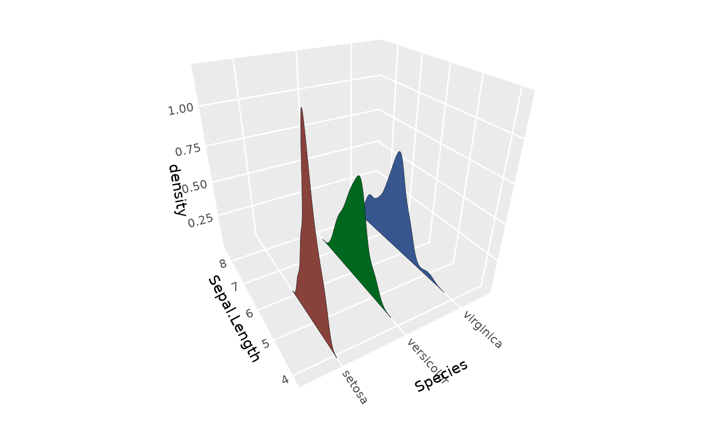
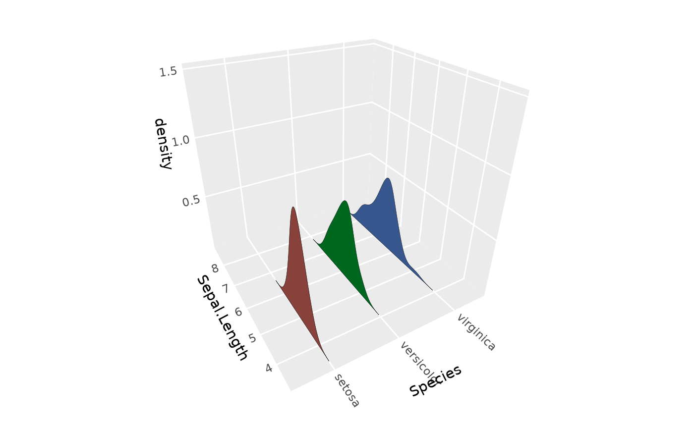
# Basic usage with iris data
p <- ggplot(iris, aes(y = Sepal.Length, x = Species, fill = Species)) +
coord_3d() +
scale_z_continuous(expand = expansion(mult = c(0, NA))) + # remove gap beneath ridges
theme(legend.position = "none")
p + stat_distributions_3d()
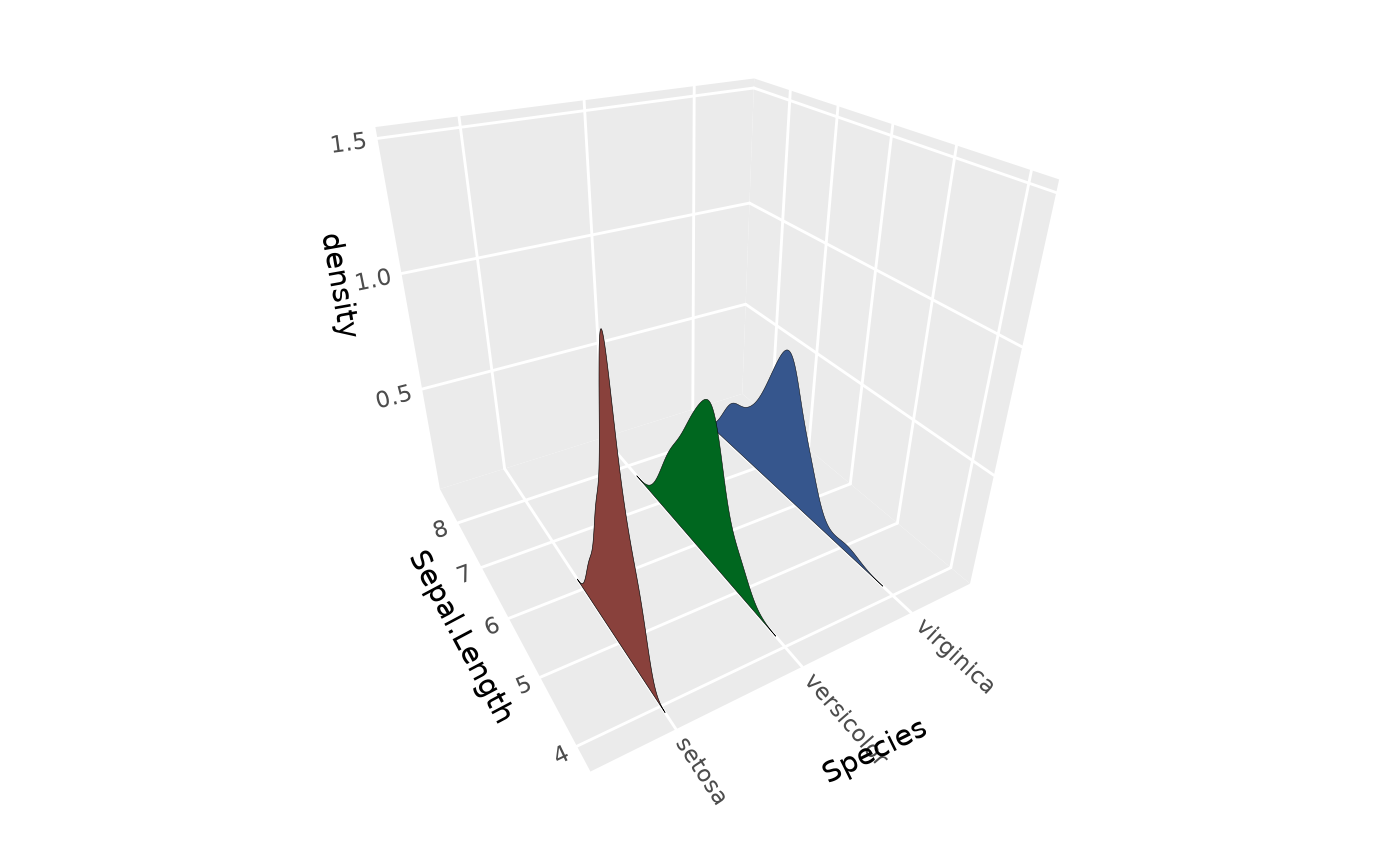
 # Normalize max ridge heights
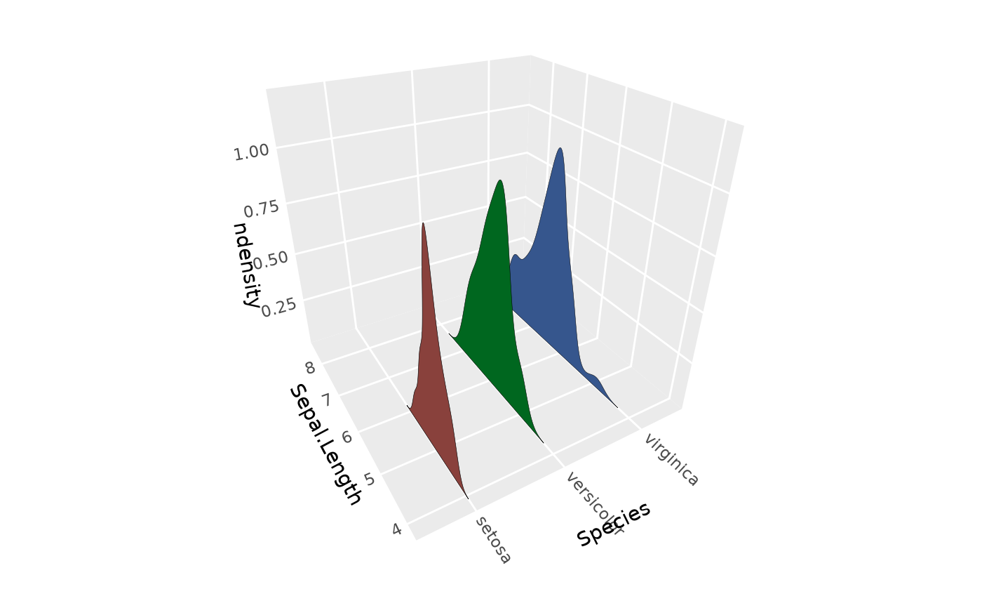
p + stat_distributions_3d(aes(z = after_stat(ndensity)))
# Normalize max ridge heights
p + stat_distributions_3d(aes(z = after_stat(ndensity)))
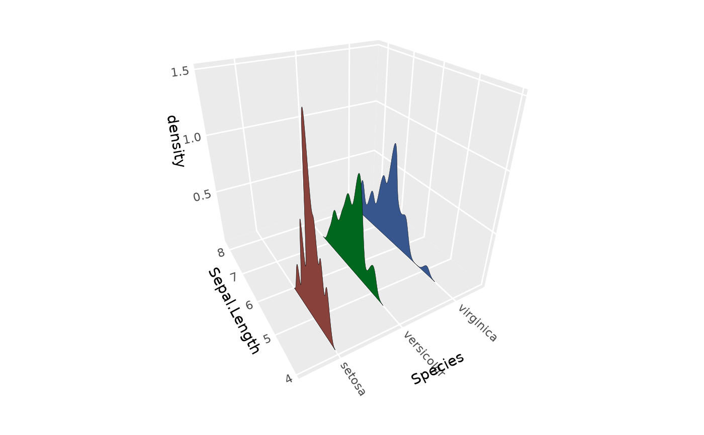
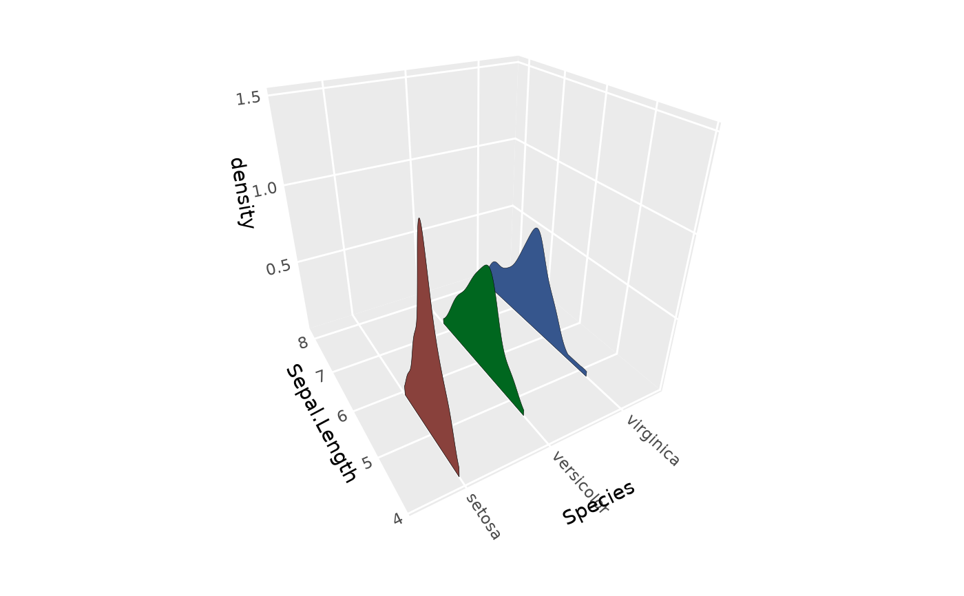
 # Adjust smoothing bandwidth
p + stat_distributions_3d(adjust = 0.5)
# Adjust smoothing bandwidth
p + stat_distributions_3d(adjust = 0.5)
 # Use joint bandwidth for consistent smoothing across groups
p + stat_distributions_3d(joint_bandwidth = TRUE)
#> Picking joint bandwidth of 0.274
# Use joint bandwidth for consistent smoothing across groups
p + stat_distributions_3d(joint_bandwidth = TRUE)
#> Picking joint bandwidth of 0.274
 # Different bandwidth selection rules
p + stat_distributions_3d(bw = "SJ")
# Different bandwidth selection rules
p + stat_distributions_3d(bw = "SJ")
 # Remove tails with rel_min_height
p + stat_distributions_3d(rel_min_height = 0.05)
# Remove tails with rel_min_height
p + stat_distributions_3d(rel_min_height = 0.05)
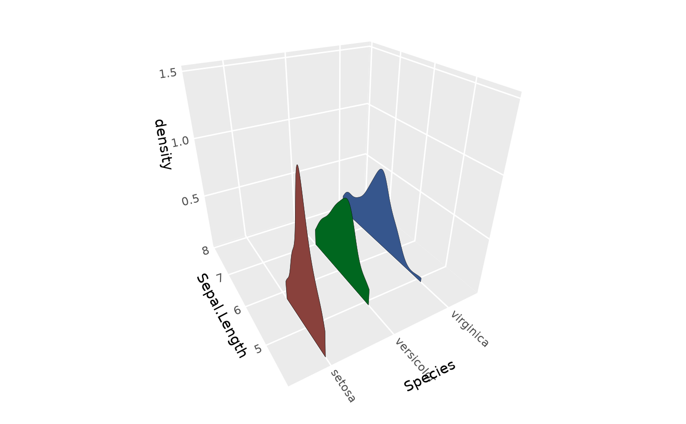
 # Trim to data range
p + stat_distributions_3d(trim = TRUE)
# Trim to data range
p + stat_distributions_3d(trim = TRUE)
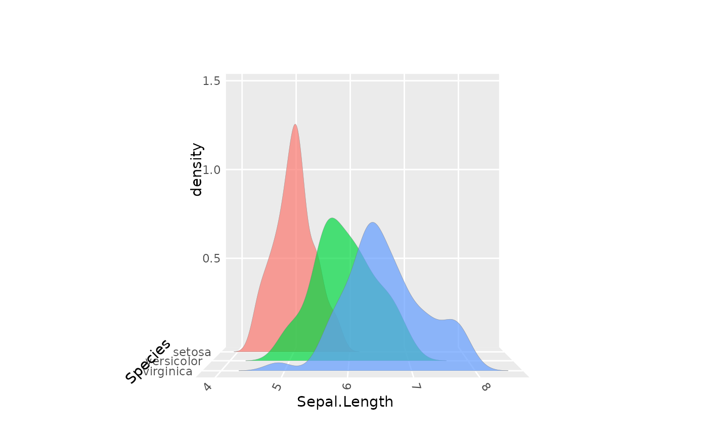
 # Rotated to reduce perspective distortion
p + stat_distributions_3d(alpha = .7) +
coord_3d(pitch = 0, roll = -90, yaw = 90, dist = 5,
panels = c("zmin", "xmin"))
#> Coordinate system already present.
#> ℹ Adding new coordinate system, which will replace the existing one.
# Rotated to reduce perspective distortion
p + stat_distributions_3d(alpha = .7) +
coord_3d(pitch = 0, roll = -90, yaw = 90, dist = 5,
panels = c("zmin", "xmin"))
#> Coordinate system already present.
#> ℹ Adding new coordinate system, which will replace the existing one.