A 3D version of ggplot2::stat_density_2d().
Creates surfaces from 2D point data using kernel density estimation.
The density values become the z-coordinates of the surface, allowing
visualization of data concentration as peaks and valleys in 3D space.
Usage
geom_density_3d(
  mapping = NULL,
  data = NULL,
  stat = "density_3d",
  position = "identity",
  ...,
  grid = "rectangle",
  n = 40,
  direction = "x",
  trim = TRUE,
  h = NULL,
  adjust = 1,
  pad = 0.1,
  min_ndensity = 0,
  light = NULL,
  cull_backfaces = FALSE,
  sort_method = NULL,
  force_convex = FALSE,
  scale_depth = TRUE,
  na.rm = FALSE,
  show.legend = NA,
  inherit.aes = TRUE
)

stat_density_3d(
  mapping = NULL,
  data = NULL,
  geom = "surface_3d",
  position = "identity",
  ...,
  grid = "rectangle",
  n = 40,
  direction = "x",
  trim = TRUE,
  h = NULL,
  adjust = 1,
  pad = 0.1,
  min_ndensity = 0,
  light = NULL,
  cull_backfaces = FALSE,
  sort_method = NULL,
  force_convex = FALSE,
  scale_depth = TRUE,
  na.rm = FALSE,
  show.legend = NA,
  inherit.aes = TRUE
)
Arguments
- mapping
Set of aesthetic mappings created by
aes(). This stat requiresxandyaesthetics. By default,fillis mapped toafter_stat(density)andzis mapped toafter_stat(density).- data
The data to be displayed in this layer. Must contain x and y columns with point coordinates.
- stat
The statistical transformation to use on the data. Defaults to
StatDensity3D.- position
Position adjustment, defaults to "identity". To collapse the result onto one 2D surface, use
position_on_face().- ...
Other arguments passed on to the layer function (typically GeomPolygon3D), such as aesthetics like
colour,fill,linewidth,annotate = annotate_3d(...), etc.- grid, n, direction, trim
Parameters determining the geometry, resolution, and orientation of the surface grid. See grid_generation for details.
- h
Bandwidth vector. If
NULL(default), uses automatic bandwidth selection viaMASS::bandwidth.nrd(). Can be a single number (used for both dimensions) or a vector of length 2 for different bandwidths in x and y directions.- adjust
Multiplicative bandwidth adjustment factor. Values greater than 1 produce smoother surfaces; values less than 1 produce more detailed surfaces. Default is 1.
- pad
Proportional range expansion factor. The computed density grid extends this proportion of the raw data range beyond each data limit. Default is 0.1.
- min_ndensity
Lower cutoff for normalized density (computed variable
ndensitydescribed below), below which to filter out results. This is particularly useful for removing low-density corners of rectangular density grids when density surfaces are shown for multiple groups, as in the example below. Default is 0 (no filtering).- light
A lighting specification object created by
light(),"none"to disable lighting, orNULLto inherit plot-level lighting specs from the coord. Specify plot-level lighting incoord_3d()and layer-specific lighting ingeom_*3d()functions.- cull_backfaces
Logical indicating whether to remove back-facing polygons from rendering. This is primarily for performance optimization but may be useful for aesthetic reasons in some situations. Backfaces are determined using screen-space winding order after 3D transformation. Defaults vary by geometry type: FALSE for open surface-type geometries, TRUE for solid objects (hulls, voxels, etc. where backfaces are generally hidden unless frontfaces are transparent or explicitly disabled).
- sort_method
Depth sorting algorithm. See sorting_methods for details.
- force_convex
Logical indicating whether to remove polygon vertices that are not part of the convex hull. Default value varies by geom. Specifying TRUE can help reduce artifacts in surfaces that have polygon tiles that wrap over a visible horizon. For prism-type geoms like columns and voxels, FALSE is safe because polygons fill always be convex.
- scale_depth
Logical indicating whether polygon linewidths should be scaled to make closer lines wider and farther lines narrower. Default is TRUE. Scaling is based on the mean depth of a polygon.
- na.rm
If
FALSE, missing values are removed.- show.legend
Logical indicating whether this layer should be included in legends.
- inherit.aes
If
FALSE, overrides the default aesthetics.- geom
The geometric object used to display the data. Defaults to
GeomPolygon3D.
Aesthetics
stat_density_3d() requires the following aesthetics from input data:
x: X coordinate of data points
y: Y coordinate of data points
And optionally understands:
group: Grouping variable for computing separate density surfaces
Additional aesthetics are passed through for surface styling
Computed variables specific to StatDensity3D
density: The kernel density estimate at each grid pointndensity: Density estimate scaled to maximum of 1 within each groupcount: Density estimate × number of observations in group (expected count)n: Number of observations in each group
Grouping
When aesthetics like colour or fill are mapped to categorical variables,
stat_density_3d() computes separate density surfaces for each group, just
like stat_density_2d(). Each group gets its own density calculation with
proper count and n values.
Computed variables
The following computed variables are available via after_stat():
x,y,z: Grid coordinates and function valuesnormal_x,normal_y,normal_z: Surface normal componentsslope: Gradient magnitude from surface calculationsaspect: Direction of steepest slope from surface calculationsdzdx,dzdy: Partial derivatives from surface calculation
See also
ggplot2::stat_density_2d() for 2D density contours, stat_surface_3d() for
surfaces from existing grid data, light() for lighting specifications,
coord_3d() for 3D coordinate systems.
Examples
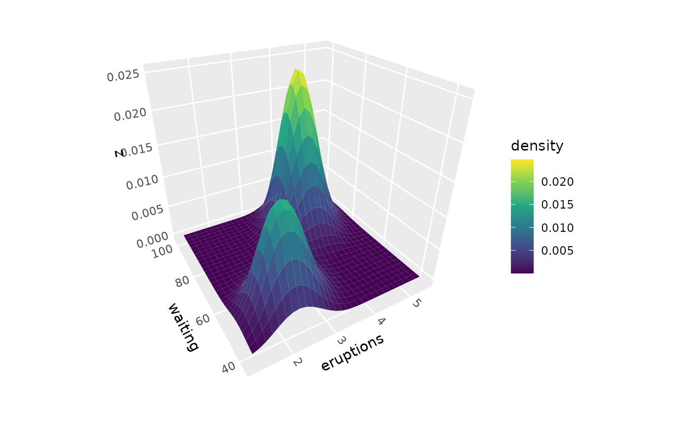
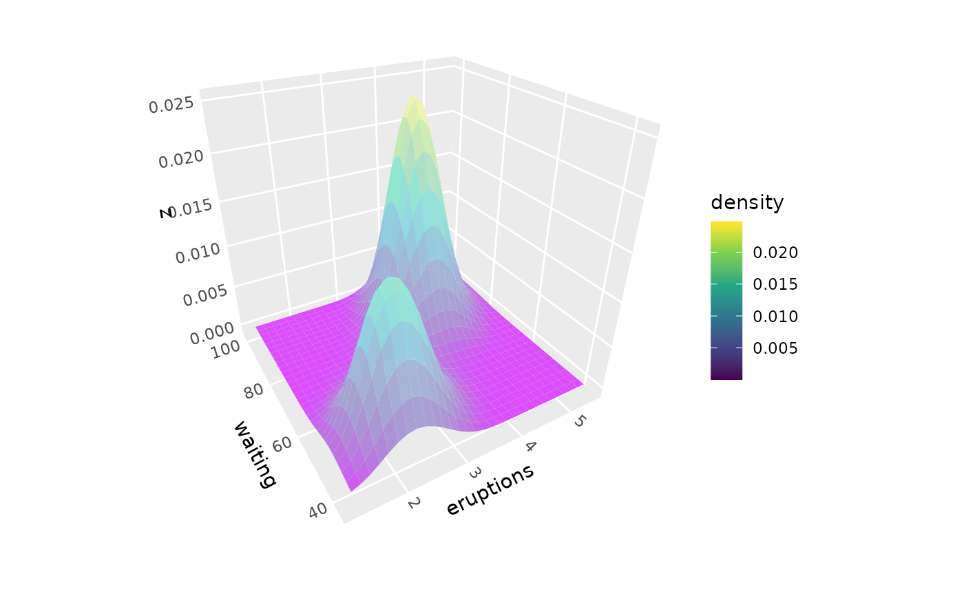
# Basic density surface from scattered points
p <- ggplot(faithful, aes(eruptions, waiting)) +
coord_3d() +
scale_fill_viridis_c()
p + geom_density_3d() + guides(fill = guide_colorbar_3d())
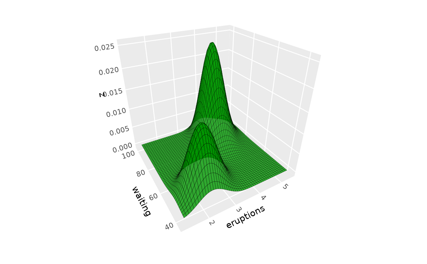
 # \donttest{
# Specify alternative grid geometry and light model
p + geom_density_3d(grid = "equilateral", n = 30, direction = "y",
light = light("direct"),
color = "white", linewidth = .1) +
guides(fill = guide_colorbar_3d())
# \donttest{
# Specify alternative grid geometry and light model
p + geom_density_3d(grid = "equilateral", n = 30, direction = "y",
light = light("direct"),
color = "white", linewidth = .1) +
guides(fill = guide_colorbar_3d())
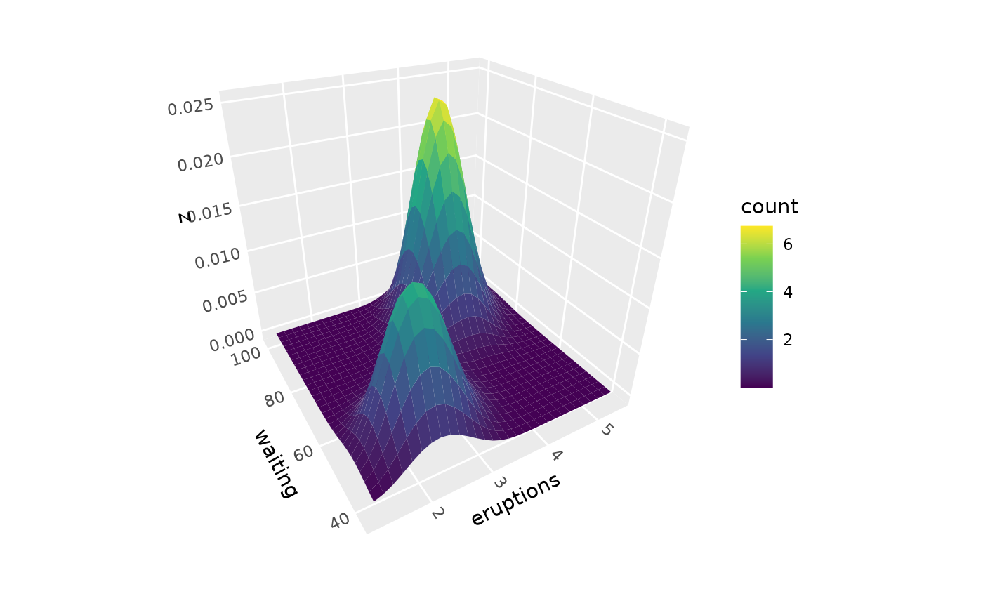 # Color by alternative density metric
p + geom_density_3d(aes(fill = after_stat(count)))
# Color by alternative density metric
p + geom_density_3d(aes(fill = after_stat(count)))
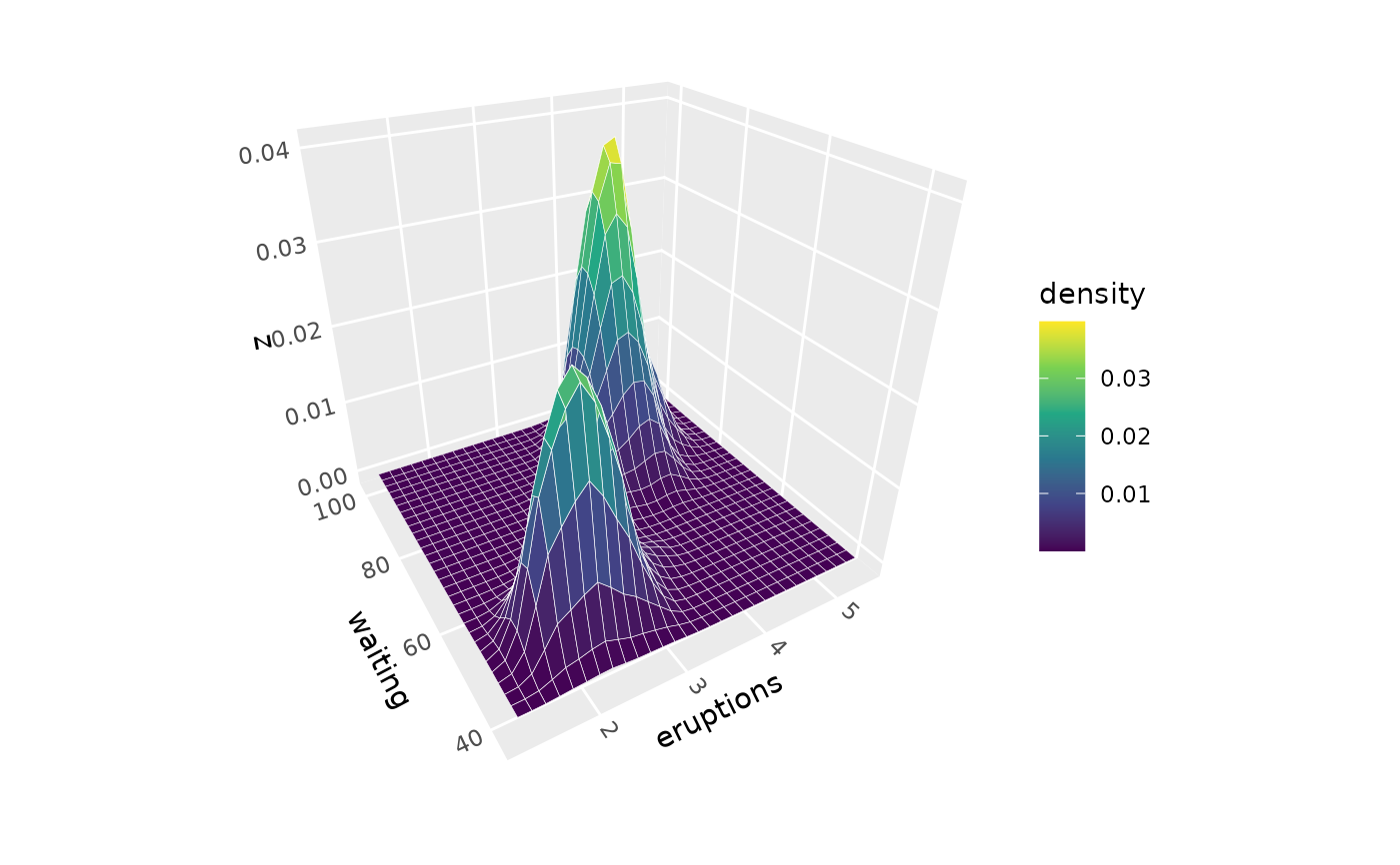 # Adjust bandwidth for smoother or more detailed surfaces
p + geom_density_3d(adjust = 0.5, n = 100, color = "white") # More detail
# Adjust bandwidth for smoother or more detailed surfaces
p + geom_density_3d(adjust = 0.5, n = 100, color = "white") # More detail
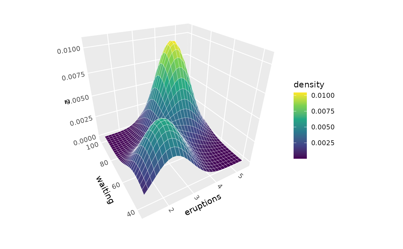 p + geom_density_3d(adjust = 2, color = "white") # Smoother
 # As contour plot instead of default surface plot
p + stat_density_3d(geom = "contour_3d", light = "none",
color = "black", bins = 25,
sort_method = "pairwise")
# As contour plot instead of default surface plot
p + stat_density_3d(geom = "contour_3d", light = "none",
color = "black", bins = 25,
sort_method = "pairwise")
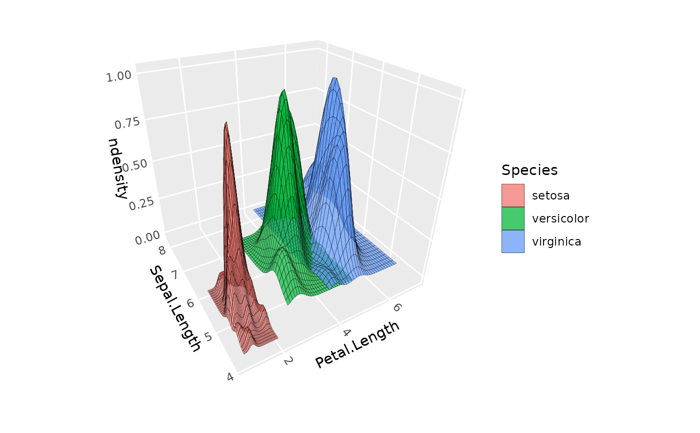
 # Multiple density surfaces by group,
# using normalized density to equalize peak heights
ggplot(iris, aes(Petal.Length, Sepal.Length, fill = Species)) +
geom_density_3d(aes(z = after_stat(ndensity), group = Species),
color = "black", alpha = .7, light = NULL) +
coord_3d()
# Multiple density surfaces by group,
# using normalized density to equalize peak heights
ggplot(iris, aes(Petal.Length, Sepal.Length, fill = Species)) +
geom_density_3d(aes(z = after_stat(ndensity), group = Species),
color = "black", alpha = .7, light = NULL) +
coord_3d()
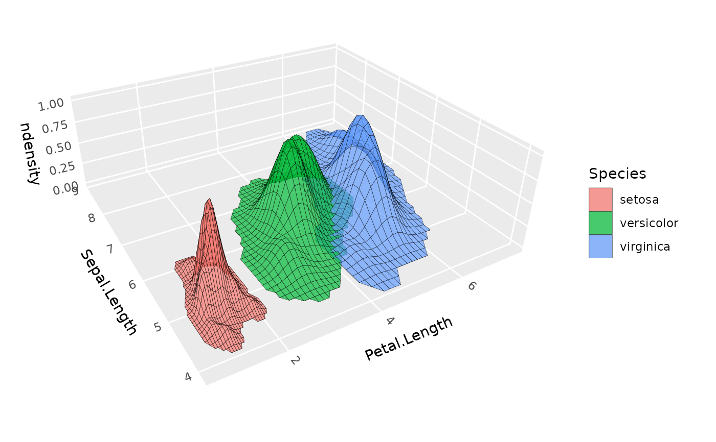
 # Same, but with extra padding to remove edge effects and
# with density filtering to remove rectangular artifacts
ggplot(iris, aes(Petal.Length, Sepal.Length, fill = Species)) +
geom_density_3d(aes(z = after_stat(ndensity)),
pad = .3, min_ndensity = .001,
color = "black", alpha = .7, light = NULL) +
coord_3d(ratio = c(3, 3, 1))
# Same, but with extra padding to remove edge effects and
# with density filtering to remove rectangular artifacts
ggplot(iris, aes(Petal.Length, Sepal.Length, fill = Species)) +
geom_density_3d(aes(z = after_stat(ndensity)),
pad = .3, min_ndensity = .001,
color = "black", alpha = .7, light = NULL) +
coord_3d(ratio = c(3, 3, 1))
 # }
# }