Convert occurrence point data to a gridded community data set

This function takes a set of occurrence point localities (e.g. from GBIF or BIEN) and rasterizes them onto a spatial grid to produce a community data set suitable for passing to phylospatial(). Each species' point records are aggregated within grid cells to produce either binary presence-absence or count data.

Usage

ps_grid(
  x,
  grid = NULL,
  res = NULL,
  crs = NULL,
  cols = c(1, 2, 3),
  data_type = c("binary", "count")
)

Arguments

x: A data frame or sf points object containing occurrence records. If a data frame, it must contain columns for species identity and geographic coordinates (see cols). Coordinates in a data frame are assumed to be WGS84 longitude and latitude; an error is thrown if values fall outside valid ranges. If an sf object, it must contain a column for species identity and have point geometry; only the first element of cols is used.
grid: An optional SpatRaster to use as the target grid. If provided, res and crs are ignored. Point records falling outside the grid extent are silently dropped.
res: Numeric giving the grid cell resolution when generating a new grid. Units are meters if crs is provided or auto-generated, or in the units of crs otherwise. Ignored if grid is provided. If NULL (the default), a resolution is automatically chosen to produce approximately 1000 grid cells across the extent of the data. See Details.
crs: Optional CRS specification (any format accepted by terra::crs()) for the output grid. Ignored if grid is provided. If NULL (the default), an Albers Equal Area projection centered on the data is automatically generated. See Details.
cols: A vector of length 1 (for sf input) or 3 (for data frame input) identifying the columns in x for species, longitude, and latitude, in that order. Can be character column names or integer column indices but not a mix. Default is c(1, 2, 3). For sf input, only the first element (species column) is used; the remaining elements are ignored.
data_type: Character indicating the type of community data to produce. Either "binary" (default), in which cells receive a 1 if one or more records are present and 0 otherwise, or "count", in which cells receive the number of records.

Value

A SpatRaster with one layer per species, suitable for passing directly to phylospatial() as the comm argument. Layer names correspond to unique values in the species column.

Details

When grid is NULL, a grid is automatically generated from the point data. If crs is also NULL, an Albers Equal Area (AEA) projection is created based on the geographic extent of the points, with the central meridian and latitude at the midpoint of the coordinate ranges, and standard parallels at 1/6 and 5/6 of the latitude range. This ensures that grid cells are equal-area, which is an assumption of various functions in the phylospatial package. Users working with other spatial layers (e.g., environmental rasters) may want to supply a grid or crs that matches their existing data.

When res is NULL and no grid is supplied, the resolution is automatically chosen so that the grid contains approximately 1000 cells. Specifically, the resolution is set to sqrt(extent_area / 1000), where extent_area is the area of the bounding box of the projected points. The auto-generated grid is buffered by half a grid cell on each side to ensure that edge points are not excluded.

The res parameter is interpreted in the units of the output CRS. When the auto-generated AEA projection is used, units are meters. If a geographic (lon/lat) CRS is supplied, res is in degrees and the resulting cells will not be equal-area; a warning is issued in this case.

Coordinate cleaning and taxonomic name matching are outside the scope of this function. Users are encouraged to clean occurrence data beforehand (e.g., using the CoordinateCleaner package) and to ensure that species names in the occurrence data match the tip labels of their phylogeny before proceeding to phylospatial().

Examples

# \donttest{
# simulate some occurrence records
set.seed(42)
occ <- data.frame(
  species = sample(paste0("sp", 1:10), 500, replace = TRUE),
  x = runif(500, -122, -118),
  y = runif(500, 34, 38)
)

# grid the occurrences with auto resolution (~1000 cells)
comm <- ps_grid(occ)
#> Grid resolution set to 12639 (in CRS units) to target ~1000 cells.
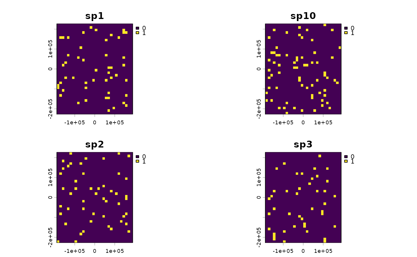
terra::plot(comm[[1:4]])


# specify columns by name
comm <- ps_grid(occ, cols = c("species", "x", "y"))
#> Grid resolution set to 12639 (in CRS units) to target ~1000 cells.

# grid at a specific resolution (50 km)
comm <- ps_grid(occ, res = 50000)

# use a custom grid
template <- terra::rast(res = 0.5, xmin = -123, xmax = -117, ymin = 33, ymax = 39,
                        crs = "EPSG:4326")
comm2 <- ps_grid(occ, grid = template)

# from sf points
occ_sf <- sf::st_as_sf(occ, coords = c("x", "y"), crs = 4326)
comm3 <- ps_grid(occ_sf, cols = "species")
#> Grid resolution set to 12639 (in CRS units) to target ~1000 cells.
# }