Creates 3D bar charts by automatically counting discrete data or binning continuous data.
This is the 3D analogue of ggplot2::geom_bar() and ggplot2::geom_histogram().
Usage
geom_bar_3d(
  mapping = NULL,
  data = NULL,
  stat = StatBar3D,
  position = "identity",
  ...,
  bins = 10,
  binwidth = NULL,
  drop = TRUE,
  width = 1,
  faces = "all",
  light = NULL,
  cull_backfaces = TRUE,
  sort_method = NULL,
  scale_depth = TRUE,
  force_convex = FALSE,
  na.rm = FALSE,
  show.legend = NA,
  inherit.aes = TRUE
)

stat_bar_3d(
  mapping = NULL,
  data = NULL,
  geom = GeomPolygon3D,
  position = "identity",
  ...,
  bins = 10,
  binwidth = NULL,
  drop = TRUE,
  width = 1,
  faces = "all",
  light = NULL,
  cull_backfaces = TRUE,
  sort_method = NULL,
  scale_depth = TRUE,
  force_convex = FALSE,
  na.rm = FALSE,
  show.legend = NA,
  inherit.aes = TRUE
)
Arguments
- mapping
Set of aesthetic mappings created by
aes().- data
The data to be displayed in this layer.
- stat
The statistical transformation to use. Defaults to
StatBar3D.- position
Position adjustment, defaults to "identity". To collapse the result onto one 2D surface, use
position_on_face().- ...
Other arguments passed on to the layer function (typically GeomPolygon3D), such as aesthetics like
colour,fill,linewidth,annotate = annotate_3d(...), etc.- bins
Number of bins in each dimension. Either a single value (used for both x and y) or a vector of length 2 giving
c(bins_x, bins_y). Default is 10. Ignored for discrete variables.- binwidth
Bin width in each dimension. Either a single value or a vector of length 2 giving
c(binwidth_x, binwidth_y). If provided, overridesbins. Ignored for discrete variables.- drop
If
TRUE(the default), empty bins/combinations are not rendered. IfFALSE, empty bins render as zero-height columns.- width
Column width as a fraction of bin spacing. Either a single value (used for both x and y) or a vector of length 2 giving
c(width_x, width_y). Default is 1.0 (columns touch). Use values less than 1 for gaps between columns.- faces
Character vector specifying which faces to render. Options:
"all"(default): Render all 6 faces"none": Render no facesVector of face names:
c("zmax", "xmin", "ymax"), etc.
Valid face names: "xmin", "xmax", "ymin", "ymax", "zmin", "zmax". Note that this setting acts jointly with backface culling, which removes faces whose interior faces the viewer – e.g., when
cull_backfaces = TRUEandfaces = "all"(the default), only front faces are rendered.- light
A lighting specification object created by
light(),"none"to disable lighting, orNULLto inherit plot-level lighting specs from the coord. Specify plot-level lighting incoord_3d()and layer-specific lighting ingeom_*3d()functions.- cull_backfaces
Logical indicating whether to remove back-facing polygons from rendering. This is primarily for performance optimization but may be useful for aesthetic reasons in some situations. Backfaces are determined using screen-space winding order after 3D transformation. Defaults vary by geometry type: FALSE for open surface-type geometries, TRUE for solid objects (hulls, voxels, etc. where backfaces are generally hidden unless frontfaces are transparent or explicitly disabled).
- sort_method
Depth sorting algorithm. See sorting_methods for details.
- scale_depth
Logical indicating whether polygon linewidths should be scaled to make closer lines wider and farther lines narrower. Default is TRUE. Scaling is based on the mean depth of a polygon.
- force_convex
Logical indicating whether to remove polygon vertices that are not part of the convex hull. Default value varies by geom. Specifying TRUE can help reduce artifacts in surfaces that have polygon tiles that wrap over a visible horizon. For prism-type geoms like columns and voxels, FALSE is safe because polygons fill always be convex.
- na.rm
If
FALSE, missing values are removed.- show.legend
Logical indicating whether this layer should be included in legends.
- inherit.aes
If
FALSE, overrides the default aesthetics.- geom
The geometric object used to display the data. Defaults to
GeomPolygon3D.
Details
The stat automatically detects whether x and y are discrete or continuous:
Both discrete: Counts occurrences of each (x, y) combination
Both continuous: Performs 2D binning (like a 3D histogram)
Mixed: Bins the continuous axis while preserving discrete groups
For pre-computed bar heights, use geom_col_3d() instead.
Aesthetics
stat_bar_3d() requires the following aesthetics:
x: X coordinate
y: Y coordinate
And optionally understands:
weight: Observation weights for counting
Computed variables
These variables can be used with after_stat() to map to aesthetics:
count: Number of observations in each bin (default for z)proportion: Count divided by total count (sums to 1)ncount: Count scaled to maximum of 1density: Count divided by (total count × bin area); integrates to 1 for continuous datandensity: Density scaled to maximum of 1
See also
geom_col_3d() for pre-computed heights, coord_3d() for 3D coordinate systems,
light() for lighting specifications.
Examples
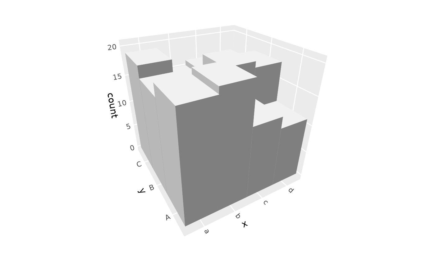
# Discrete x and y: count combinations
d_discrete <- data.frame(
x = sample(letters[1:4], 200, replace = TRUE),
y = sample(LETTERS[1:3], 200, replace = TRUE)
)
ggplot(d_discrete, aes(x, y)) +
geom_bar_3d() +
coord_3d()
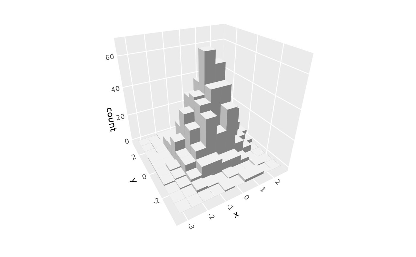
 # Continuous x and y: 2D histogram
d_cont <- data.frame(x = rnorm(1000), y = rnorm(1000))
ggplot(d_cont, aes(x, y)) +
geom_bar_3d() +
coord_3d()
# Continuous x and y: 2D histogram
d_cont <- data.frame(x = rnorm(1000), y = rnorm(1000))
ggplot(d_cont, aes(x, y)) +
geom_bar_3d() +
coord_3d()
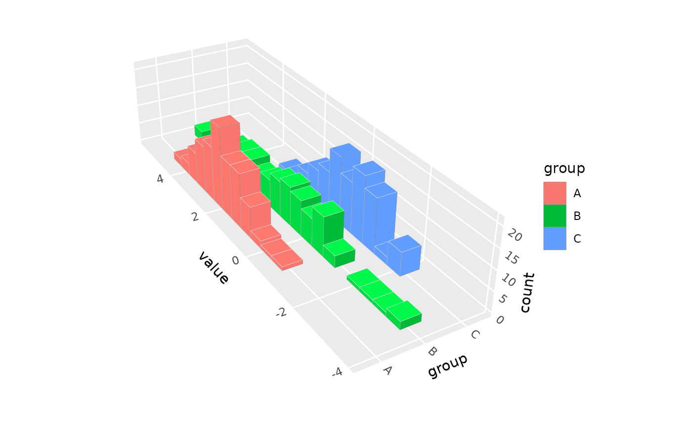
 # Mixed: one discrete, one continuous
d_mixed <- data.frame(
group = rep(c("A", "B", "C"), each = 100),
value = c(rnorm(100, 2), rnorm(100, 1, 2), rnorm(100, 0))
)
ggplot(d_mixed, aes(x = group, y = value, fill = group)) +
geom_bar_3d(bins = 20, width = c(.5, 1)) +
coord_3d(scales = "fixed", ratio = c(1, 1, .1))
# Mixed: one discrete, one continuous
d_mixed <- data.frame(
group = rep(c("A", "B", "C"), each = 100),
value = c(rnorm(100, 2), rnorm(100, 1, 2), rnorm(100, 0))
)
ggplot(d_mixed, aes(x = group, y = value, fill = group)) +
geom_bar_3d(bins = 20, width = c(.5, 1)) +
coord_3d(scales = "fixed", ratio = c(1, 1, .1))
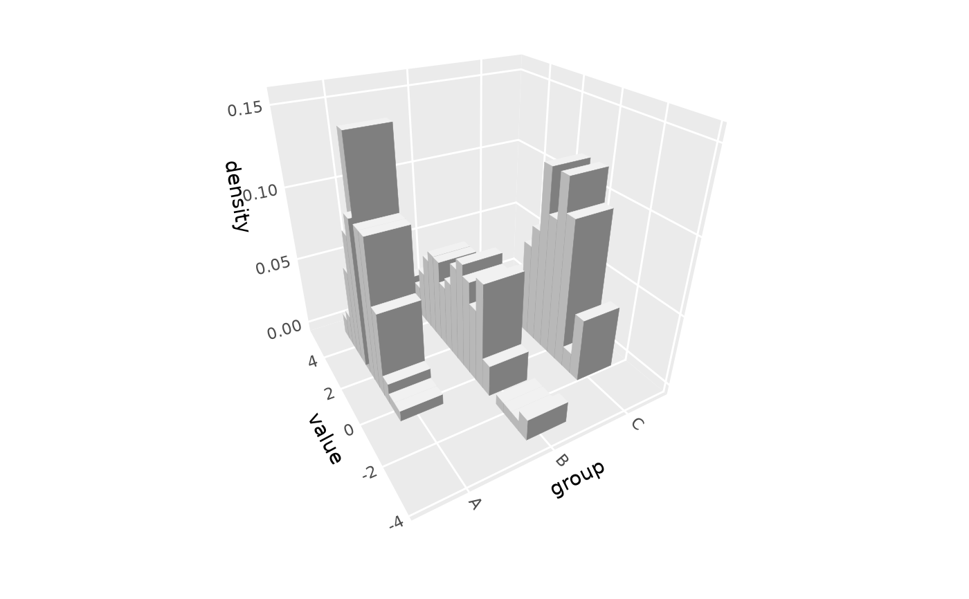
 # Use density instead of count for z
ggplot(d_mixed,
aes(x = group, y = value, z = after_stat(density))) +
geom_bar_3d(bins = 20, width = c(.5, 1)) +
coord_3d()
# Use density instead of count for z
ggplot(d_mixed,
aes(x = group, y = value, z = after_stat(density))) +
geom_bar_3d(bins = 20, width = c(.5, 1)) +
coord_3d()
 # Show empty bins with drop = FALSE
ggplot(d_cont, aes(x, y)) +
geom_bar_3d(drop = FALSE) +
coord_3d()
# Show empty bins with drop = FALSE
ggplot(d_cont, aes(x, y)) +
geom_bar_3d(drop = FALSE) +
coord_3d()