Introduction to nullcat

library(nullcat)

Introduction

nullcat provides null model algorithms for categorical and quantitative community ecology data. It extends classic binary null models (e.g., curveball, swap) to work with categorical data, and introduces a stratified randomization framework for continuous data.

Categorical null models generalize binary null models to matrices where cells contain integers representing discrete categories. Whereas binary models preserve totals (e.g. row or column sums), categorical models preserve multisets (e.g. category frequencies in each row or column). For example, if a row contains [1, 1, 2, 3, 3, 3], a row-preserving categorical algorithm would preserve this exact multiset—two 1s, one 2, and three 3s—while randomizing where these categories appear within the row.

Traditional binary models are simply the specific two-category cases of their corresponding general categorical models (e.g. curveball is equivalent to curvecat with only two categories).

Use cases

Categorical null models are designed for cell-level categorical data—characteristics of a species at a site—rather than site-level or species-level attributes. They can be useful for categorical and ordinal ecological data. Examples include:

Ordinal states: phenological stages, health status, life stages
Multi-state interactions: interaction type, infection status, mutualism outcomes
Population genetic states: genotypes or allelic frequencies at the population level
Binned quantitative measures: abundance classes, cover scales, or occurrence probability bins (the quantize() function covered below automates binning and randomization)
Binary data: species presence-absence data or similar

Categorical null models

Available algorithms

The package provides five categorical null model algorithms:

curvecat(): Categorical curveball (most efficient)
swapcat(): Categorical 2×2 swap
tswapcat(): Categorical trial-swap
r0cat(): Row-constrained randomization
c0cat(): Column-constrained randomization

Example: Basic categorical randomization

# Create a categorical matrix
set.seed(123)
x <- matrix(sample(1:4, 100, replace = TRUE), nrow = 10)

# Randomize using curvecat (preserves row & column category multisets)
x_rand <- curvecat(x, n_iter = 1000)

# Verify margins are preserved
all.equal(sort(x[1, ]), sort(x_rand[1, ]))  # Row preserved
#> [1] TRUE
all.equal(sort(x[, 1]), sort(x_rand[, 1]))  # Column preserved
#> [1] TRUE

Understanding fixed margins

Different algorithms preserve different margins:

set.seed(456)
x <- matrix(sample(1:3, 60, replace = TRUE), nrow = 10)

# Fixed-fixed: both row and column margins preserved
x_fixed <- curvecat(x, n_iter = 1000)

# Row-constrained: only row margins preserved
x_row <- r0cat(x)

# Column-constrained: only column margins preserved
x_col <- c0cat(x)

# Check row sums by category
table(x[1, ])           # Original row 1
#> 
#> 1 2 3 
#> 2 2 2
table(x_fixed[1, ])     # Preserved in curvecat
#> 
#> 1 2 3 
#> 2 2 2
table(x_row[1, ])       # Preserved in r0cat
#> 
#> 1 2 3 
#> 2 2 2
table(x_col[1, ])       # Not preserved in c0cat
#> 
#> 1 2 3 
#> 1 3 2

Quantitative null models

The quantize() function provides stratified randomization for continuous community data (abundance, biomass, cover, occurrence probability). It works by applying the following steps:

Stratify: use a flexible binning scheme to convert continuous values into discrete strata
Randomize: apply one of the categorical null models described above to the stratified matrix
Reassign: map randomized strata back to original values, subject to a chosen constraint

Why use quantize? Existing quantitative null models lack flexibility in what margins they preserve. While binary curveball elegantly preserves row and column totals, and vegan’s quasiswap models do this for count data, there’s no framework for preserving row and/or column value distributions for continuous data (abundance, biomass, cover). The stratification approach fills this gap: when using fixed = "row" or fixed = "col", one dimension’s value multisets are preserved exactly while the other is preserved at the resolution of strata. This is the closest available approximation to a quantitative fixed-fixed null model. Additionally, stratification provides explicit control over the preservation-randomization tradeoff through the number of strata used.

Example: Basic quantitative randomization

# Create a quantitative community matrix
set.seed(789)
comm <- matrix(runif(200), nrow = 20)

# Default: curvecat-backed stratified randomization with 5 strata
rand1 <- quantize(comm, n_strata = 5, n_iter = 2000, fixed = "row")

# Values are similar but rearranged
cor(as.vector(comm), as.vector(rand1))
#> [1] 0.1757922
plot(rowSums(comm), rowSums(rand1))

plot(colSums(comm), colSums(rand1))

Stratification options

When you call quantize(), it uses the helper function stratify() to convert your continuous data to discrete bins. The stratification scheme can strongly influence your randomization results, because it is frequencies of these categories that are constrained during matrix permutation. By default, data are split into a handful of equal-width bins, but this can be controlled with parameters including n_strata, transform, zero_stratum, breaks, and offset. Let’s call stratify() directly here, to understand its behavior—a good idea for a real analysis, not just a tutorial.

set.seed(200)
x <- rexp(100, .1)

# More strata = less mixing, higher fidelity to original distribution
s3 <- stratify(x, n_strata = 3)
s10 <- stratify(x, n_strata = 10)

table(s3)   # Coarser bins
#> s3
#>  1  2  3 
#> 89  9  2
table(s10)  # Finer bins
#> s10
#>  1  2  3  4  5  6 10 
#> 49 22 17  4  4  2  2

# Transform before stratifying (e.g., log-transform for skewed data)
s_log <- stratify(x, n_strata = 5, transform = log1p)
table(s_log)
#> s_log
#>  1  2  3  4  5 
#> 14 26 27 27  6

# Rank transform creates equal-occupancy strata
s_rank <- stratify(x, n_strata = 5, transform = rank)
table(s_rank)  # Nearly equal counts per stratum
#> s_rank
#>  1  2  3  4  5 
#> 20 20 20 20 20

# Separate zeros into their own stratum
x_with_zeros <- c(0, 0, 0, x)
s_zero <- stratify(x_with_zeros, n_strata = 4, zero_stratum = TRUE)
table(s_zero)
#> s_zero
#>  1  2  3  4 
#>  3 89  9  2

Controlling what’s preserved

While the mechanics of the chosen randomization algorithm determine which margins of the randomized categories are preserved, the fixed parameter controls how the original continuous values are mapped back onto the randomized categories, determining which margins preserve their original value distributions. There are four options for the fixed parameter: row, col, cell, and stratum, though only a subset of these are relevant for some algorithms. For a method like the default curvecat algorithm that preserves both row and column categorical multisets, all four are available:

set.seed(100)
comm <- matrix(rexp(100), nrow = 10)

# Preserve row value multisets (quantitative row sums maintained)
rand_row <- quantize(comm, n_strata = 5, fixed = "row", n_iter = 2000)
all.equal(rowSums(comm), rowSums(rand_row))
#> [1] TRUE

# Preserve column value multisets (quantitative column sums maintained)
rand_col <- quantize(comm, n_strata = 5, fixed = "col", n_iter = 2000)
all.equal(colSums(comm), colSums(rand_col))
#> [1] TRUE

# Cell-level preservation: each value moves with its original cell location
# The categorical randomization determines WHERE cells go, but each cell
# carries its original value with it
rand_cell <- quantize(comm, n_strata = 5, fixed = "cell", n_iter = 2000)

# Values shuffled globally within strata, holding none of the above fixed
rand <- quantize(comm, n_strata = 5, fixed = "stratum", n_iter = 2000)

# For non-fixed-fixed methods like r0cat or c0cat, only some fixed options make sense:
# r0cat with fixed="col" or c0cat with fixed="row" would be incompatible

Efficient repeated randomization

The quantize routine includes some setup, including stratification, that doesn’t need to be repeatedly recomputed when generating multiple randomized versions of the same matrix. For generating null distributions, you can pre-compute overhead once using quantize_prep(), or you can use *_batch() functions to efficiently generate multiple replicates (optionally using parallel processing).

set.seed(400)
comm <- matrix(rexp(200), nrow = 20)

# Prepare once
prep <- quantize_prep(comm, n_strata = 5, fixed = "row", n_iter = 2000)

# Generate many randomizations efficiently
rand1 <- quantize(prep = prep)
rand2 <- quantize(prep = prep)
rand3 <- quantize(prep = prep)

# Or use batch functions
nulls <- quantize_batch(comm, n_reps = 99, n_strata = 5, 
                       fixed = "row", n_iter = 2000)
dim(nulls)  # 20 rows × 10 cols × 99 replicates
#> [1] 20 10 99

Convergence diagnostics

Sequential algorithms (curvecat, swapcat, tswapcat) require sufficient iterations to reach stationarity. You can use the trace_cat() function with either nullcat or quantize to assess how many iterations are needed for your particular dataset and algorithm. The trace shows how similarity to the original matrix changes over iterations; when the trace stabilizes around zero, the algorithm has reached stationarity. You can also use suggest_n_iter() to get an automated suggestion for a reasonable number of burn-in iterations to reach stationarity.

set.seed(300)
x <- matrix(sample(1:5, 400, replace = TRUE), nrow = 20)

# Generate trace showing mixing over iterations
trace <- trace_cat(x, fun = "nullcat", method = "curvecat",
                   n_iter = 1000, n_chains = 3, thin = 10)

# Visual inspection
plot(trace)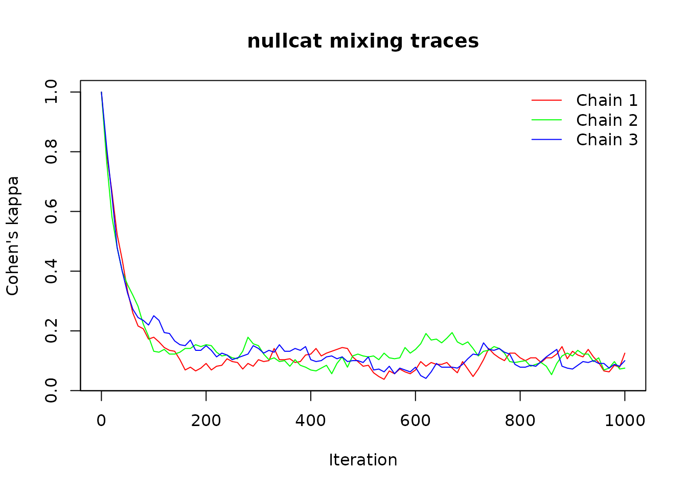


# Automatic burn-in suggestion
suggested <- suggest_n_iter(trace, tail_frac = 0.3)
print(suggested)
#> suggested_n_iter object
#> -----------------------
#> Converged: TRUE 
#> Suggested n iterations: 410

Integration with `vegan`

nullcat includes several functions to integrate with the vegan package’s null model framework. For both nullcat() and quantize(), there are sequential and non-sequential variants of these functions that create vegan::commsim() objects suitable for use with vegan::nullmodel() and vegan::oecosimu(). Examples include:

library(vegan)

# Categorical data
x_cat <- matrix(sample(1:4, 100, replace = TRUE), nrow = 10)
cs <- nullcat_commsim_seq(method = "curvecat")
nm <- nullmodel(x_cat, cs)
sims <- simulate(nm, nsim = 99, burnin = 1000, thin = 100)

# Quantitative data
x_quant <- matrix(rexp(100), nrow = 10)
cs_quant <- quantize_commsim(n_strata = 5, method = "curvecat", n_iter = 2000)
nm_quant <- nullmodel(x_quant, cs_quant)
sims_quant <- simulate(nm_quant, nsim = 99)

References

Strona et al. (2014). A fast and unbiased procedure to randomize ecological binary matrices. Nature Communications, 5, 4114.
Gotelli (2000). Null model analysis of species co-occurrence patterns. Ecology, 81(9), 2606-2621.