Takes user-provided (x, y, z) point data and prepares it for surface rendering. If data form a regular grid, can render either a GeomSurface3D of rectangular or right-triangular tiles, or a GeomRidgeline3D or GeomContour3D set of surface slices; otherwise, renders irregular triangular tiles via Delaunay trianuglation.
Usage
stat_surface_3d(
  mapping = NULL,
  data = NULL,
  geom = "surface_3d",
  position = "identity",
  ...,
  cull_backfaces = FALSE,
  light = NULL,
  na.rm = FALSE,
  show.legend = NA,
  inherit.aes = TRUE
)

geom_surface_3d(
  mapping = NULL,
  data = NULL,
  stat = "surface_3d",
  position = "identity",
  ...,
  method = "auto",
  grid = NULL,
  cull_backfaces = FALSE,
  sort_method = "auto",
  scale_depth = TRUE,
  force_convex = TRUE,
  light = NULL,
  na.rm = FALSE,
  show.legend = NA,
  inherit.aes = TRUE
)
Arguments
- mapping
Set of aesthetic mappings created by
aes(). Must includex,y, andz. By default, fill is mapped toafter_stat(z).- data
Data frame containing point coordinates.
- geom
Geom to use for rendering. Defaults to
"surface_3d"for mesh surfaces. Use"ridgeline_3d"for ridgeline rendering.- position
Position adjustment, defaults to "identity".
- ...
Other arguments passed to the layer.
- cull_backfaces
Logical indicating whether to remove back-facing polygons from rendering. This is primarily for performance optimization but may be useful for aesthetic reasons in some situations. Backfaces are determined using screen-space winding order after 3D transformation. Defaults vary by geometry type: FALSE for open surface-type geometries, TRUE for solid objects (hulls, voxels, etc. where backfaces are generally hidden unless frontfaces are transparent or explicitly disabled).
- light
A lighting specification object created by
light(),"none"to disable lighting, orNULLto inherit plot-level lighting specs from the coord. Specify plot-level lighting incoord_3d()and layer-specific lighting ingeom_*3d()functions.- na.rm
If
FALSE, missing values are removed.- show.legend
Logical indicating whether this layer should be included in legends.
- inherit.aes
If
FALSE, overrides the default aesthetics.- stat
Statistical transformation to use on the data. Defaults to
"surface_3d".- method
Tessellation method passed to
geom_surface_3d(): "auto" (default), "grid", or "delaunay".- grid
Tile geometry for regular grids: "rectangle" (default), "right1", or "right2".
- sort_method
Depth sorting algorithm. See sorting_methods for details.
- scale_depth
Logical indicating whether polygon linewidths should be scaled to make closer lines wider and farther lines narrower. Default is TRUE. Scaling is based on the mean depth of a polygon.
- force_convex
Logical indicating whether to remove polygon vertices that are not part of the convex hull. Default value varies by geom. Specifying TRUE can help reduce artifacts in surfaces that have polygon tiles that wrap over a visible horizon. For prism-type geoms like columns and voxels, FALSE is safe because polygons fill always be convex.
Details
For regular grids, computes point-level gradients. Works with
both geom_surface_3d() for mesh rendering and geom_ridgeline_3d() for
ridgeline rendering.
Computed variables
For regular grid data:
- dzdx, dzdy
Partial derivatives at each point
- slope
Gradient magnitude: sqrt(dzdx^2 + dzdy^2)
- aspect
Direction of steepest slope: atan2(dzdy, dzdx)
For irregular data, gradient variables are NA.
Grid detection
The stat automatically detects whether data forms a regular grid by checking
if nrow(data) == length(unique(x)) * length(unique(y)). Regular grids
get point-level gradient computation; irregular point clouds are passed
through for Delaunay tessellation by the geom.
See also
geom_surface_3d(), geom_ridgeline_3d(), stat_function_3d(),
coord_3d()
Examples
# Regular grid data ------------------------------------------
# simulated data and base plot for basic surface
d <- dplyr::mutate(tidyr::expand_grid(x = -10:10, y = -10:10),
z = sqrt(x^2 + y^2) / 1.5,
z = cos(z) - z)
p <- ggplot(d, aes(x, y, z)) +
coord_3d(light = light(mode = "hsl", direction = c(1, 0, 0)))
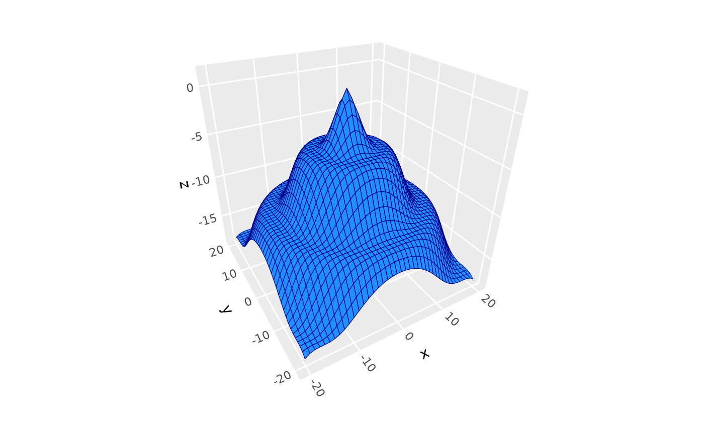
# surface with 3d lighting
p + geom_surface_3d(fill = "steelblue", color = "steelblue", linewidth = .2)
 # \donttest{
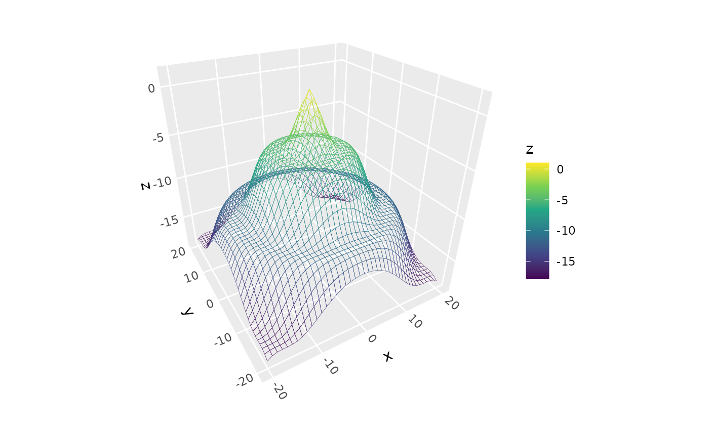
# mesh wireframe (`fill = NA`) with aes line color
p + geom_surface_3d(aes(color = z), fill = NA,
linewidth = .5, light = "none") +
scale_color_gradientn(colors = c("black", "blue", "red"))
# \donttest{
# mesh wireframe (`fill = NA`) with aes line color
p + geom_surface_3d(aes(color = z), fill = NA,
linewidth = .5, light = "none") +
scale_color_gradientn(colors = c("black", "blue", "red"))
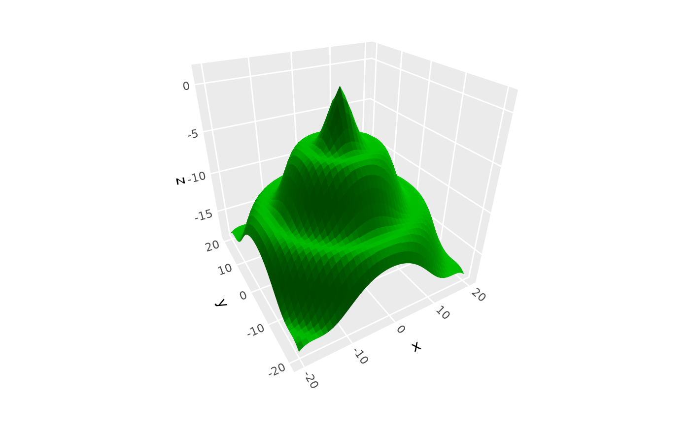 # triangulated surface (can prevent lighting flaws)
p + geom_surface_3d(fill = "#9e2602", color = "black", grid = "right2")
# triangulated surface (can prevent lighting flaws)
p + geom_surface_3d(fill = "#9e2602", color = "black", grid = "right2")
 # use after_stat to access computed surface-orientation variables
p + geom_surface_3d(aes(fill = after_stat(slope)), grid = "right2") +
scale_fill_viridis_c() +
guides(fill = guide_colorbar_3d())
# use after_stat to access computed surface-orientation variables
p + geom_surface_3d(aes(fill = after_stat(slope)), grid = "right2") +
scale_fill_viridis_c() +
guides(fill = guide_colorbar_3d())
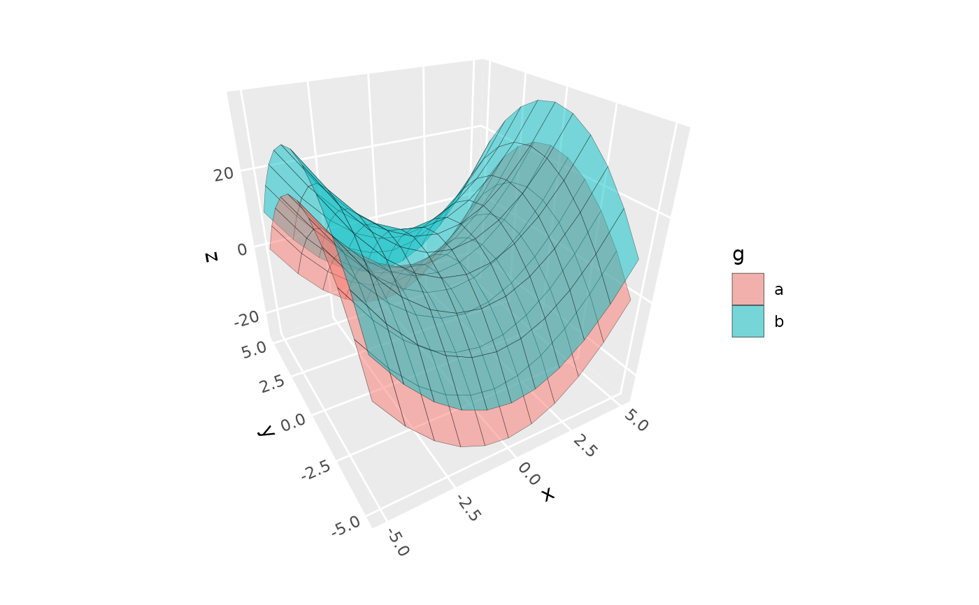 # use `group` to plot data for multiple surfaces
d <- expand.grid(x = -5:5, y = -5:5)
d$z <- d$x^2 - d$y^2
d$g <- "a"
d2 <- d
d2$z <- d$z + 15
d2$g <- "b"
ggplot(rbind(d, d2), aes(x, y, z, group = g, fill = g)) +
coord_3d(light = "none") +
geom_surface_3d(color = "black", alpha = .5, light = NULL)
# use `group` to plot data for multiple surfaces
d <- expand.grid(x = -5:5, y = -5:5)
d$z <- d$x^2 - d$y^2
d$g <- "a"
d2 <- d
d2$z <- d$z + 15
d2$g <- "b"
ggplot(rbind(d, d2), aes(x, y, z, group = g, fill = g)) +
coord_3d(light = "none") +
geom_surface_3d(color = "black", alpha = .5, light = NULL)
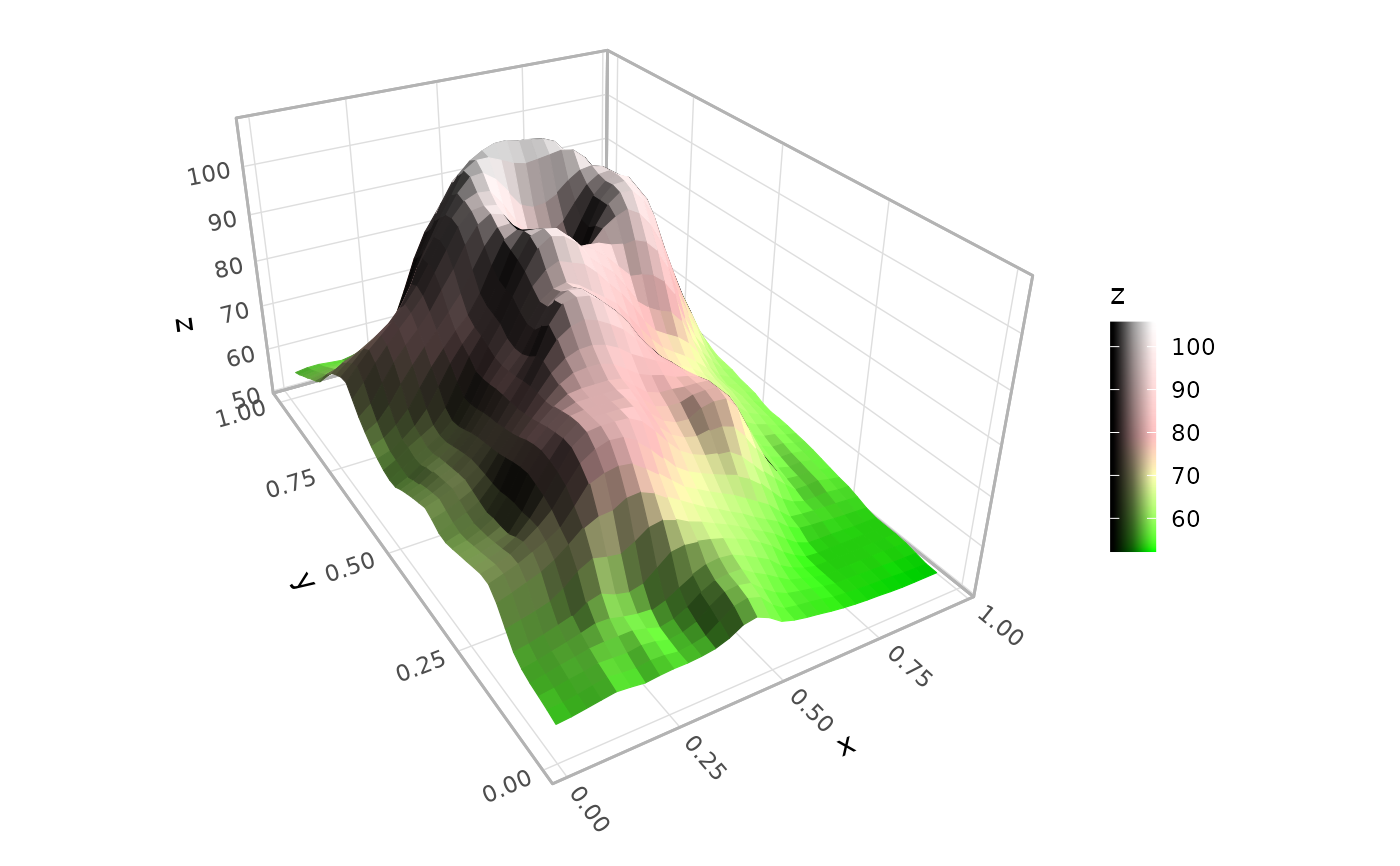
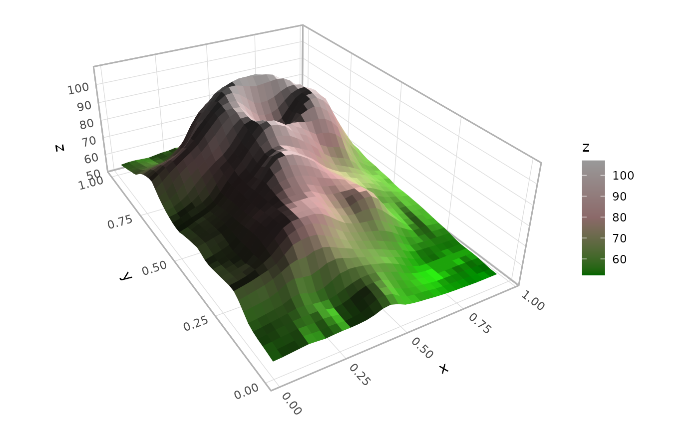 # terrain surface with topographic hillshade and elevational fill
ggplot(mountain, aes(x, y, z, fill = z, color = z)) +
geom_surface_3d(light = light(direction = c(1, 0, .5),
mode = "hsv", contrast = 1.5),
linewidth = .2) +
coord_3d(ratio = c(1, 1.5, .75)) +
theme_light() +
scale_fill_gradientn(colors = c("darkgreen", "rosybrown4", "gray60")) +
scale_color_gradientn(colors = c("darkgreen", "rosybrown4", "gray60")) +
guides(fill = guide_colorbar_3d())
# terrain surface with topographic hillshade and elevational fill
ggplot(mountain, aes(x, y, z, fill = z, color = z)) +
geom_surface_3d(light = light(direction = c(1, 0, .5),
mode = "hsv", contrast = 1.5),
linewidth = .2) +
coord_3d(ratio = c(1, 1.5, .75)) +
theme_light() +
scale_fill_gradientn(colors = c("darkgreen", "rosybrown4", "gray60")) +
scale_color_gradientn(colors = c("darkgreen", "rosybrown4", "gray60")) +
guides(fill = guide_colorbar_3d())
 # stack of flat surfaces (e.g. a time series of raster maps)
d <- expand.grid(lon = 1:20, lat = 1:20, time = 1:6)
d$value <- sin(-d$lon * d$lat / 10) + d$time / 2
ggplot(d, aes(lon, lat, time, group = time,
fill = value, color = value)) +
geom_surface_3d(light = "none") +
coord_3d() +
scale_color_viridis_c() + scale_fill_viridis_c()
# stack of flat surfaces (e.g. a time series of raster maps)
d <- expand.grid(lon = 1:20, lat = 1:20, time = 1:6)
d$value <- sin(-d$lon * d$lat / 10) + d$time / 2
ggplot(d, aes(lon, lat, time, group = time,
fill = value, color = value)) +
geom_surface_3d(light = "none") +
coord_3d() +
scale_color_viridis_c() + scale_fill_viridis_c()
 # stat_surface_3d with alternative geoms ----------------------------
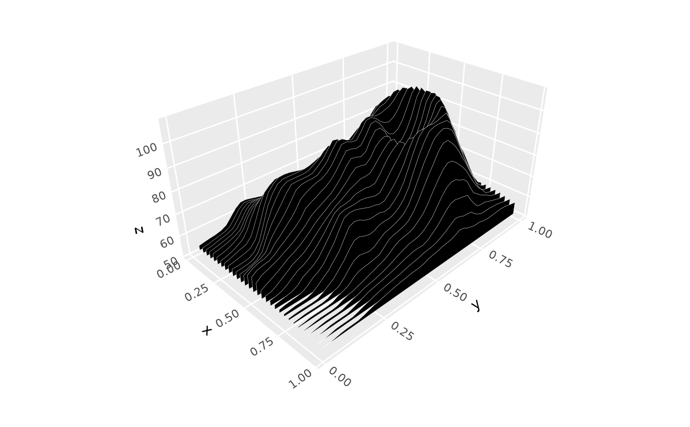
# horizontal slices with geom_ridgeline_3d
ggplot(mountain, aes(x, y, z)) +
stat_surface_3d(geom = "ridgeline_3d",
fill = "black", color = "white",
light = "none", linewidth = .1) +
coord_3d(ratio = c(1, 1.5, .75), yaw = 45)
# stat_surface_3d with alternative geoms ----------------------------
# horizontal slices with geom_ridgeline_3d
ggplot(mountain, aes(x, y, z)) +
stat_surface_3d(geom = "ridgeline_3d",
fill = "black", color = "white",
light = "none", linewidth = .1) +
coord_3d(ratio = c(1, 1.5, .75), yaw = 45)
 # elevation contours with geom_contour_3d
ggplot(mountain, aes(x, y, z, fill = z)) +
stat_surface_3d(geom = "contour_3d", light = "none",
bins = 25, sort_method = "pairwise",
color = "black") +
coord_3d(ratio = c(1, 1.5, .75), yaw = 45) +
scale_fill_viridis_c(option = "B")
# elevation contours with geom_contour_3d
ggplot(mountain, aes(x, y, z, fill = z)) +
stat_surface_3d(geom = "contour_3d", light = "none",
bins = 25, sort_method = "pairwise",
color = "black") +
coord_3d(ratio = c(1, 1.5, .75), yaw = 45) +
scale_fill_viridis_c(option = "B")
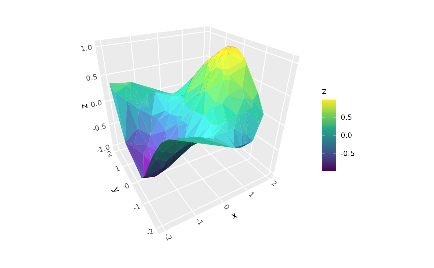
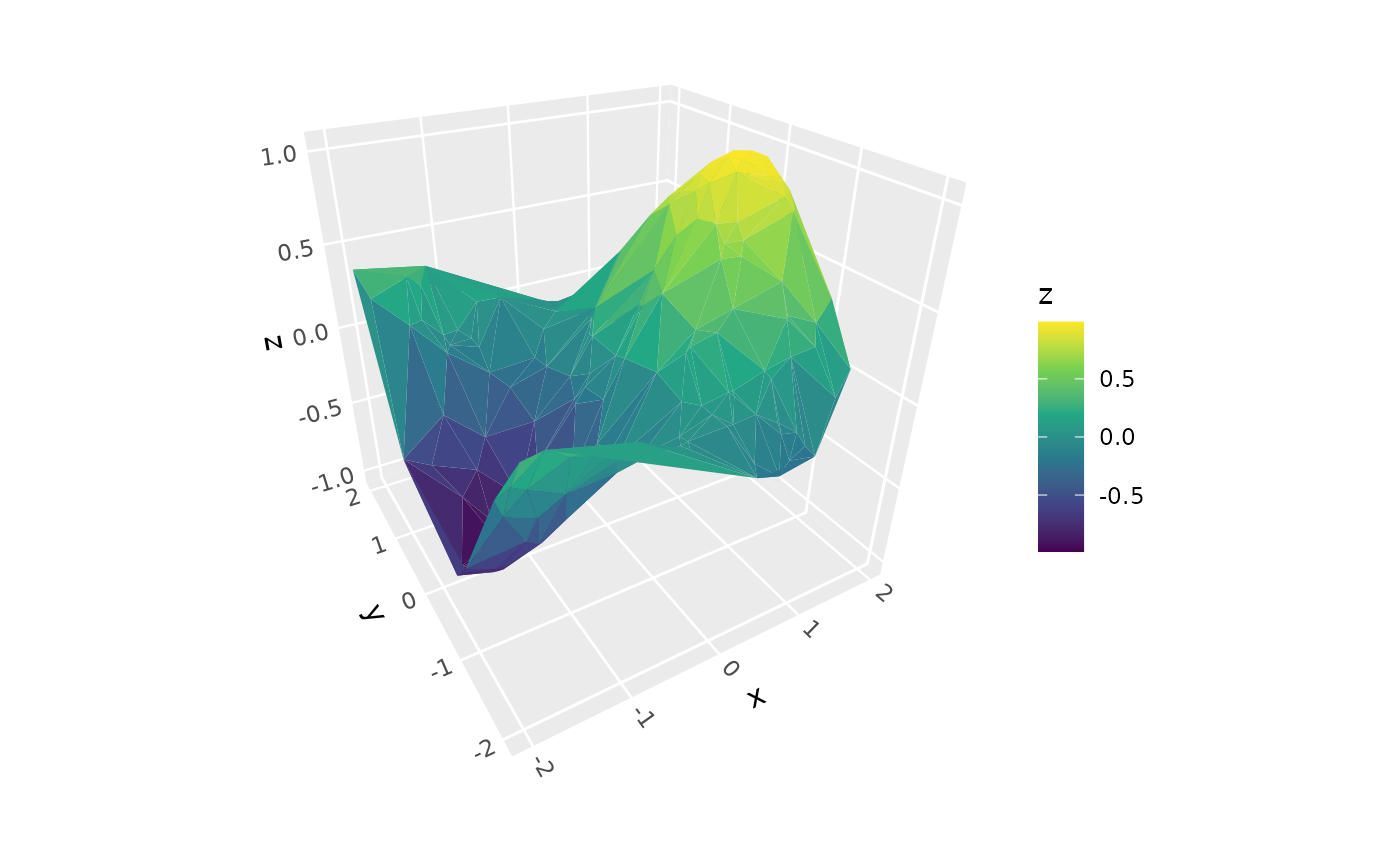
 # Irregular point data ---------------------------------------
set.seed(42)
pts <- data.frame(x = runif(200, -2, 2), y = runif(200, -2, 2))
pts$z <- with(pts, sin(x) * cos(y))
ggplot(pts, aes(x, y, z = z, fill = z)) +
stat_surface_3d(sort_method = "pairwise") +
scale_fill_viridis_c() +
coord_3d(light = "none")
# Irregular point data ---------------------------------------
set.seed(42)
pts <- data.frame(x = runif(200, -2, 2), y = runif(200, -2, 2))
pts$z <- with(pts, sin(x) * cos(y))
ggplot(pts, aes(x, y, z = z, fill = z)) +
stat_surface_3d(sort_method = "pairwise") +
scale_fill_viridis_c() +
coord_3d(light = "none")
 # }
# }