
Circuitscape and Omniscape
Source:vignettes/articles/circuitscape-omniscape.Rmd
circuitscape-omniscape.RmdThe cs_*() and os_*() functions run Circuitscape.jl
and Omniscape.jl:
circuitscaper writes their configuration files from your R arguments and
rasters, runs them in Julia, and reads the results back as terra
rasters. This article covers each mode and its options; see
vignette("getting-started") for installation, inputs and
choosing a method. For more on the methods themselves, see the Circuitscape
and Omniscape
documentation.
Circuitscape: pairwise mode
Pairwise mode solves a circuit for every pair of focal nodes, with one unit of current flowing from one to the other.
library(terra)
#> terra 1.9.27
#>
#> Attaching package: 'terra'
#> The following objects are masked from 'package:testthat':
#>
#>     compare, describe
library(circuitscaper)

# Resistance surface (higher values = harder to traverse)
resistance <- rast(system.file("extdata/resistance.tif", package = "circuitscaper"))

# Option 1: Focal nodes as coordinates (simplest)
coords <- matrix(c(10, 40, 40, 40, 10, 10, 40, 10), ncol = 2, byrow = TRUE)
result <- cs_pairwise(resistance, coords)

# Option 2: Focal nodes as a raster (integer IDs; 0 and NA are not nodes)
# locations <- rast("path/to/focal_nodes.tif")
# result <- cs_pairwise(resistance, locations)

# Cumulative current map -- high values indicate important movement corridors
plot(result$current_map)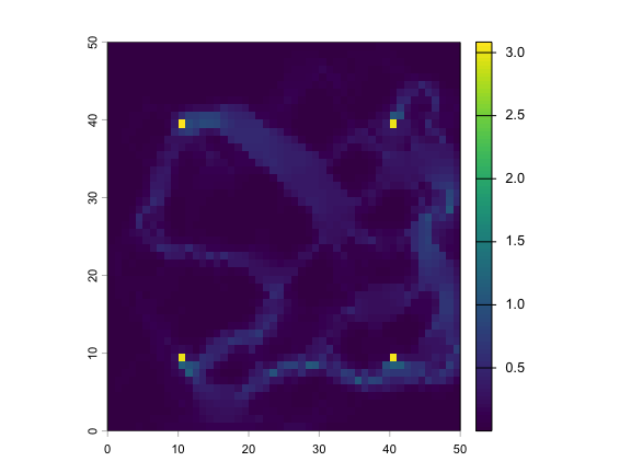
# Pairwise resistance matrix -- can be used as a connectivity distance metric
result$resistance_matrix
#>          1        2        3        4
#> 1  0.00000 22.80786 23.09078 17.39341
#> 2 22.80786  0.00000 37.00636 25.87992
#> 3 23.09078 37.00636  0.00000 24.98422
#> 4 17.39341 25.87992 24.98422  0.00000
Circuitscape: one-to-all and all-to-one modes
One-to-all mode injects current at each focal node in turn, with all the others grounded; all-to-one mode grounds each node in turn, with all the others injecting.
result <- cs_one_to_all(resistance, coords)
plot(result)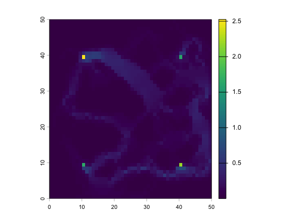
result <- cs_all_to_one(resistance, coords)
plot(result$cumulative_current)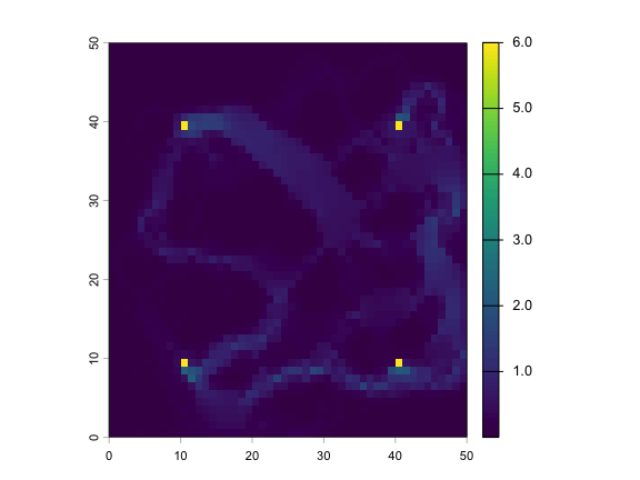
Circuitscape: advanced mode
Advanced mode takes explicit source current and ground conductance rasters and solves one circuit.
source_layer <- rast(system.file("extdata/source.tif", package = "circuitscaper"))
ground_layer <- rast(system.file("extdata/ground.tif", package = "circuitscaper"))

result <- cs_advanced(resistance, source_layer, ground_layer,
                      ground_is = "conductances")

# Current density -- corridors and pinch points where flow is concentrated,
# i.e. possible preservation priorities
# Voltage -- analogous to movement probability, decreasing with distance
# and resistance from sources
# Power dissipation -- areas of current flow through high-resistance areas,
# i.e. possible restoration priorities
power <- result[["current"]]^2 * resistance
plot(c(result[["current"]], result[["voltage"]], power), nc = 3,
     main = c("current", "voltage", "power"))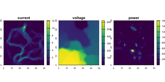
Additional Circuitscape options
Per-pair current and voltage maps
By default, pairwise, one-to-all, and all-to-one modes return only
the cumulative current map. Set cumulative_only = FALSE to
include per-pair (or per-node) current layers, and
write_voltage = TRUE to include voltage layers:
result <- cs_pairwise(resistance, coords,
                      cumulative_only = FALSE,
                      write_voltage = TRUE)
names(result$current_map)
#>  [1] "cumulative_current" "current_1_2"        "current_1_3"
#>  [4] "current_1_4"        "current_2_3"        "current_2_4"
#>  [7] "current_3_4"        "voltage_1_2"        "voltage_1_3"
#> [10] "voltage_1_4"        "voltage_2_3"        "voltage_2_4"
#> [13] "voltage_3_4"
Variable source strengths
By default, each focal node injects 1 amp of current. Use
source_strengths to assign different injection strengths
per node — useful when sites differ in population size or habitat
area:
# Strengths in the same order as the locations
strengths <- c(2.5, 1.0, 0.5, 1.0)
result <- cs_one_to_all(resistance, coords, source_strengths = strengths)
Short-circuit regions
Short-circuit regions represent areas of zero resistance (e.g., lakes that can be crossed freely, or developed areas that funnel movement). Pass a raster where cells sharing the same positive integer value are short-circuited:
polygons <- rast("path/to/short_circuit_regions.tif")
result <- cs_pairwise(resistance, coords, short_circuit = polygons)
Include/exclude pairs
For large numbers of focal nodes, you may want to restrict analysis to a subset of pairs:
result <- cs_pairwise(resistance, coords,
                      included_pairs = "path/to/pairs.txt")
Normalized current
Omniscape returns normalized current (actual current / flow potential) automatically. You can compute the equivalent for Circuitscape by running the analysis twice — once with your resistance surface and once with a uniform surface — and dividing:
result      <- cs_pairwise(resistance, coords)
result_null <- cs_pairwise(resistance * 0 + 1, coords)
normalized  <- result$current_map / result_null$current_map
plot(normalized)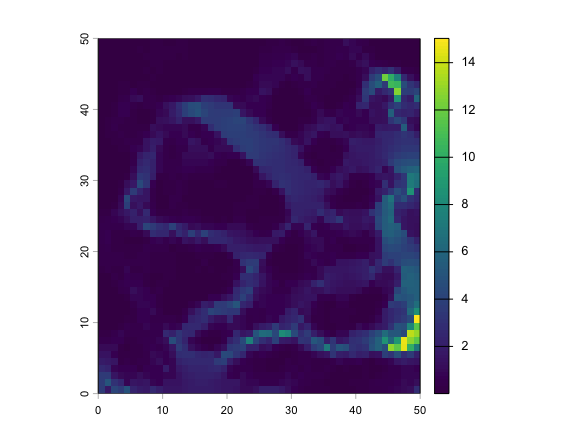
Values greater than 1 indicate areas where landscape resistance is concentrating current flow; values less than 1 indicate areas where current is lower than expected from geometry alone.
Omniscape: moving-window connectivity
Omniscape computes omnidirectional connectivity using a moving window. It does not require focal nodes — every cell can serve as a source.
The two key parameters are:
-
radius: The moving window radius in pixels. This defines the neighborhood over which connectivity is evaluated — conceptually, how far the organism can disperse. Larger radii capture longer-distance connectivity but increase computation time substantially. -
block_size: Aggregation factor for source points (default 1, no aggregation). Settingblock_size = 3groups sources into 3x3 blocks, reducing the number of circuit solves with typically negligible effects on results. This is the primary knob for trading off speed vs. precision.
result <- os_run(resistance, radius = 20, block_size = 3)Omniscape returns up to three layers:
-
cumulative_current: Raw current flow summed across all moving-window iterations. Higher values indicate cells that carry more current overall. -
flow_potential: What current flow would look like if resistance were uniform everywhere. This isolates the effect of source geometry from landscape resistance. -
normalized_current: Cumulative current divided by flow potential. Values greater than 1 indicate corridors where connectivity is higher than expected given the arrangement of sources; values less than 1 indicate relative barriers. This is usually the most informative layer.
plot(result, nc = 3)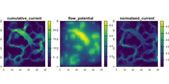
With source strength weights
By default, source strength is derived from the inverse of resistance. You can provide an explicit source strength raster (e.g., habitat quality) to weight sources independently of resistance:
Conditional connectivity
Conditional connectivity restricts which sources are connected to
each target, based on their values on a condition layer. Use
os_condition() to define the comparison. For categorical
data, type = "equal" connects only cells in the same
class:
landcover <- rast("path/to/landcover.tif")

result <- os_run(resistance, radius = 20,
                 condition = os_condition(landcover, type = "equal"))
For continuous data, lower and upper bound
the difference between source and target values. Supplying a
future layer compares each source’s present-day value
against the target’s future value, as in climate-tracking connectivity.
Here, sources connect to targets whose future temperature is between 1
degree cooler and 3 degrees warmer than the source’s present
temperature:
temp_now <- rast("path/to/temperature_current.tif")
temp_future <- rast("path/to/temperature_2080.tif")

result <- os_run(resistance, radius = 20,
                 condition = os_condition(temp_now, future = temp_future,
                                          lower = -3, upper = 1))
Up to two conditions can be combined by passing a list of
os_condition() objects; see ?os_condition for
details.
Parallel processing
For large landscapes, enable Julia multithreading to reduce compute
times. Set the number of threads with cs_setup(), ideally
at the start of your session:
Julia’s thread count is fixed when Julia starts, so if Julia is
already running with fewer threads, cs_setup(threads = 4)
restarts it. That takes about as long as the first setup, since
Circuitscape and Omniscape are loaded and warmed up again. If the
running Julia session can’t run in parallel, os_run()
warns, says how to fix it, and runs serially.
Performance
Circuitscape computation time scales with the number of non-NA cells in the resistance raster and, for focal-node modes, with the number of pairs or iterations. A few practical guidelines:
- Raster size: Problems up to ~1 million cells run comfortably. For larger landscapes, consider aggregating the resistance surface before analysis.
-
Number of focal nodes: Pairwise mode solves
n*(n-1)/2 circuits, so computation grows quadratically with the number
of nodes. Use
included_pairsto limit the set if needed, or considerdp_pairwise(), whose time hardly depends on the number of nodes. -
Omniscape: Computation is dominated by the number
of source pixels and the
radius. Useblock_sizeto reduce the source count and keepradiusas small as ecologically justified. Enableparallelize = TRUEfor large runs, or considerdp_omni(), whose time hardly depends on the radius. -
Solver choice: The default
"cg+amg"(iterative) solver works well for large problems. For small rasters (under ~10,000 cells),"cholmod"(direct solver) may be faster.
Saving outputs
By default, intermediate files are written to a temporary directory
and cleaned up. To persist output files (ASC rasters, INI configuration,
and resistance matrices), use output_dir:
result <- cs_pairwise(resistance, coords,
                      output_dir = "my_output_directory")
Set verbose = TRUE to see Circuitscape’s solver
progress, useful for debugging or monitoring long runs.