Introduction to analogs • analogs

library(analogs)
library(terra)

Overview

The analogs package implements a general framework for distance-based neighborhood models. Every analysis follows a two-stage pattern:

First, select a neighborhood of analog locations from a reference pool, based on environmental similarity, geographic proximity, or both.
Optionally, summarize the neighborhood using counts, weighted means, regression coefficients, or other statistics.

Common methods in climate change ecology—climate velocity, analog impact models, analog availability—are all specific configurations of this framework. So are geographically weighted regression (GWR) and inverse distance-weighted (IDW) interpolation, which use purely geographic neighborhoods. The package implements these via a flexible core function, analog_search(), along with simplified wrappers for common analysis types.

The table below shows how each wrapper maps to the framework:

Function	Neighborhood	Summary	Use case
`analog_velocity()`	k nearest geographic, environment-constrained	Pairs	Where is this climate moving?
`analog_similarity()`	k nearest environmental, geographically-constrained	Pairs	What climates are reachable?
`analog_availability()`	All within thresholds	Count	Where do analogs exist?
`analog_density()`	All within thresholds	Weighted sum	How strong are analog matches?
`analog_impact()`	All within thresholds	Weighted mean	What ecological conditions to expect?
`analog_regression()`	Flexible	Local regression	How do covariates predict outcomes within neighborhoods?

As described below, these functions fall into two categories: analog enumeration functions (which find analogs for each focal site and either return them directly or summarize their abundance or quality), and analog-based prediction functions (which fit local models predicting an outcome variable y observed across each focal site’s analogs). Note that while this document covers the key wrapper functions, you can also implement a broader range of analyses by calling analog_search() directly.

Data

All functions in the package require two data inputs: x (the set of focal locations for which analogs are to be found) and pool (the set of reference locations to search for analogs). Both these components need to have spatial coordinates and environmental data (most commonly climate, though other variables can also be used) for each location. Prediction functions also require y (outcome variable(s)). Data can be provided as matrices, data.frames, or SpatRasters. x and pool must have the same set of environmental variables, but can be in different formats and can represent different sets of sites.

Most of the examples in this vignette are focused on climate change, and assume that x and pool come from different time periods with different climates. In these situations, you typically have a choice about which dataset to map to which of the two parameters, and swapping them can give different insights. For example, as shown in the climate velocity section below, swapping the parameter mapping switches the analysis from forward to reverse velocity; while it’s only shown for velocity, this is also possible for the other climate change analyses. For non-climate-change applications like GWR and IDW, shown toward the end of this vignette, x and pool can be from the same time period.

The package includes an example dataset of climate rasters covering a portion of western North America at approximately 5 km resolution, with two scaled climate variables (climatic water deficit and actual evapotranspiration) for a historical baseline (1981–2010) and a future projection (2041–2070, SSP585). These are used throughout this vignette. Let’s unpack them and make some quick maps:

clim <- example_rasters()
hist <- clim$historic
fut <- clim$future

plot(hist, main = c("Historical CWD", "Historical AET"))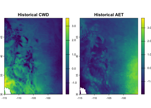

plot of chunk data

Defining analogs

Most of this document focuses on different types of analog queries. But regardless of query type, you also have to define what qualifies as an “analog.” Broadly speaking, an analog is any location in pool that is environmentally similar and/or geographically close to a given focal location in x.

Analog kernels

Your specify an analog definition using the kernel() helper function, which returns an <analog_kernel> object that can be passed to the env and geog arguments of various analog functions. Analog kernels operate on pairwise environmental and geographic distances between x and pool, which get used in two ways. Distances are used as hard thresholds to select a set of analogs, and they’re often also used as weights to place higher value on nearby/similar analogs that may be more ecologically or statistically relevant. Distance units and measures for geographic and environmental distances are thus centrally important, and are discussed below.

If you define both environmental and geographic kernels, they get intersected to define analogs.

Distance thresholds are set with the max parameter to kernel(). For example, analog_search(..., env = kernel(max = 0.25), geog = kernel(max = 100)) finds analogs within 0.25 environmental units and 100 geographic units of a given x. Note that large max values can substantially increase computation time.

Kernel weights are specified via the weight (kernel shape) and theta (kernel bandwidth) parameters. These control how analog weights decay with distance, which is relevant for some stat options. Available kernel shapes include:

"uniform" — all analogs weighted equally (also the default when weight is unspecified)
"gaussian" — Gaussian kernel with theta as standard deviation: $exp(-d^2 / (2 \times theta^2))$
"inverse" — inverse distance weighting, with theta as bandwidth: $1 / (1 + d / theta)$

When using a kernel that weights environmental and/or geographic distances, the combination of parameters should be set so that kernel weight decays to near zero at the max boundary. This allows the kernel function to drive the results while the max cutoffs function mainly to reduce run time by minimizing unneeded computation.

The helper function kernel_params() is useful for determining what values to choose for theta and max. It gives theoretical answers to the questions, “How big should theta be in order for my kernel to capture a given fraction of pool sites for the typical focal site?” and “How big should max be so that it truncates only a given percentage of kernel weight for the typical focal site?” These questions are subject to the curse of dimensionality and depend on the number of environmental variables, so intuition does not always hold. kernel_params() gives theoretical answers, assuming that pool follows a multivariate normal distribution (as approximately achieved by mahalanobis_transform()) or a uniform distribution, and that the focal site is randomly sampled from pool.

For example, if you had d = 4 environmental variables and wanted to size your Gaussian environmental kernel so that it captures 10% of the pool for the average site during the baseline era (and assuming you had run mahanobis_transform() so that your data were approximately multivariate normal), here’s how you get kernel parameter recommendations:

kernel_params(fraction = 0.10, d = 4, loss = 0.01, 
              kernel = "gaussian", data_dist = "mvn")
#> $theta
#> [1] 0.6800554
#> 
#> $max
#> [1] 2.049015

Geographic distance

The package automatically detects whether coordinates are longitude/latitude or projected, and uses great-circle or planar distance accordingly. You can override this with coord_type = "lonlat" or coord_type = "projected". Geographic thresholds are in kilometers for lon/lat data and in projection units for projected data.

Environmental distance

By default, environmental distance is Euclidean. When using multiple environmental variables, it is recommended to scale them first to avoid artifacts from differing units. The example data used here is already scaled.

For dataset-wide Mahalanobis distance (accounting for covariance among environmental variables), use mahalanobis_transform() to pre-whiten the data:

transformed <- mahalanobis_transform(x = hist, pool = fut)
vel_mahal <- analog_velocity(
      x = transformed$x,
      pool = transformed$pool,
      env = kernel(max = 0.25),
      k = 1
)

For site-specific covariance (e.g., based on local year-to-year climate variability), supply pre-computed covariance matrices via the x_cov parameter.

Analog weights

Beyond the kernel weights described above, the framework supports two other ways to weight pool sites in summary statistics. Both get multiplied through any kernel weighting and influence which analogs receive more weight in the aggregation, but do not affect which analogs are selected.

Cell-area weights correct for the fact that raster grid cells often have non-uniform area. Without correction, naive summaries over multiple analog grid cells are biased toward regions of small cells (e.g. high latitudes on a lon-lat grid, or distorted regions of a non-equal-area projection). When pool is a raster, analog functions compute and apply cell-area weights by default. You can override this with cell_area_weight = FALSE to disable it.
User weights let you express ecological or methodological variation across pool sites — for example, sampling effort, ecological intactness, occurrence probabilities for a focal species, or any other per-site weight that should influence aggregation. Pass them via the weight argument as a numeric vector, single-column matrix or data frame, or single-layer SpatRaster matching pool. Values must be non-negative; NA is allowed and is treated as zero (the site contributes nothing). User weights are reported alongside the analog index in pair-mode output, making it easy to filter or post-process based on the weight of each match.
Also note that a fourth source of weighting, sample weights, arises only when you set downsample < 1 to accelerate queries on a large pool (as discussed below). The package rescales the surviving points’ weights to keep aggregations unbiased, and these weights get multiplied with the other three. You generally do not need to think about them; they are surfaced as a sample_weight column in pair-mode output for the rare case where you want to inspect them.

Analog enumeration functions

This category of analyses includes functions that simply identify and return analogs (e.g. analog_velocity()) and functions that instead return a summary of the count or weights of analogs. Let’s look at them each in turn.

Climate velocity

Analog-based climate velocity metrics are widely used to assess dispersal constraints under climate change. Forward or outbound velocity, the distance from a site to the nearest location with a projected future climate similar to the site’s historical/current climate, represents the migration required for current residents to track baseline climate conditions. Reverse or inbound velocity, the distance from a site to the nearest location with a historical climate similar to the site’s projected future climate, represents constraints on the arrival of new residents adapted to the site’s future conditions.

These metrics are implemented as a geographic nearest-neighbor search under a hard climate constraint, with reverse velocity implemented by swapping the climate data for the two eras. For each focal site, the result returns data on its single nearest geographic analog (subject to the climate similarity threshold max). The geographic distance to that analog, divided by the time elapsed, is the velocity. Sites with no analog in the reference pool—an important category— have NA results.

fwd_vel <- analog_velocity(
      x = hist,
      pool = fut,
      env = kernel(max = 0.25),
      k = 1
)

rev_vel <- analog_velocity(
      x = fut,
      pool = hist,
      env = kernel(max = 0.25),
      k = 1
)

decades <- 6
vel <- c(fwd_vel$geog_dist, rev_vel$geog_dist) / decades
plot(vel, range = range(minmax(vel)),
     main = c("Forward velocity (km/dec)", "Reverse velocity (km/dec)"))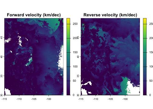

plot of chunk velocity

In addition to geographic and environmental distances, the result also includes the spatial coordinates of each site’s nearest analog (as well as the analog’s index in the pool). This can be used for a variety of downstream analyses, including visualizing the direction from a site to its analog location:

fwd_vel$bearing <- geosphere::bearing(crds(fwd_vel, na.rm = FALSE),
                                      values(fwd_vel)[, c("analog_x", "analog_y")])

plot(fwd_vel$bearing, main = c("Bearing to forward analog (deg)"),
     col = rainbow(12))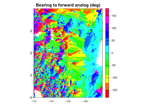

plot of chunk bearing

Environmental similarity

Environmental similarity answers the inverse question from climate velocity: for each location’s environment, what is the most similar environment within a given geographic radius? This finds the most climatically similar locations that are geographically reachable, which can provide insight into how much climate change organisms must tolerate given limited dispersal capacity.

sim <- analog_similarity(
      x = fut,
      pool = hist,
      geog = kernel(max = 100),
      k = 1
)

plot(sim$env_dist, main = "Similarity of best nearby climate analog")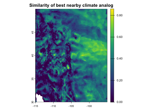

plot of chunk similarity

Analog availability

How many analogs exist within specified environmental and geographic thresholds? This maps the density of suitable analogs across the landscape. Locations with large numbers of nearby analogs have greater potential for adaptive dispersal under climate change, while locations with zero analogs represent novel or disappearing climates.

avail <- analog_availability(
      x = fut,
      pool = hist,
      env = kernel(max = 0.5),
      geog = kernel(max = 200),
)

plot(avail, main = "Analog availability (count)")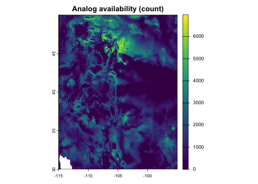

plot of chunk availability

Analog density

Similar to availability, but weighted by environmental kernel-based similarity and/or geographic proximity rather than simply counted. This captures both the quantity and quality (proximity/suitability) of analog matches. By default, raw density is normalized by dividing it by its theoretical maximum value (calculated from kernel, max_geog, and theta) to make it interpretable.

intens <- analog_density(
      x = fut,
      pool = hist,
      env = kernel(weight =  "gaussian", theta = 0.2, max = 0.6),
      geog = kernel(weight =  "gaussian", theta = 50, max = 0.25)
)

plot(intens, main = "Analog density")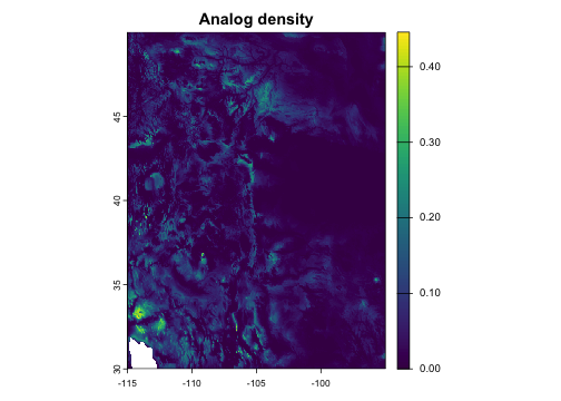

plot of chunk density

Prediction functions

Compared to the functions covered above that simply enumerate analogs, analog-based prediction functions find analogs and then fit a model that summarizes additional properties (outcome variables y) of those analogs. Model options include weighted means and categorical counts (via analog_impact()) and ordinary and ridge regression on additional covariates (via analog_regression()).

Options for assessing uncertainty include returning standard errors on fitted means and coefficients (via the se parameter) and running various forms of cross-validation within pool (via analog_cv()).

Analog impact models

Analog impact models (AIMs) predict ecological outcomes (y) under climate change. For each focal site, this approach finds locations within geographic range that have current climates similar to the focal site’s future climate, then computes an average (or class count for categorical y) of their ecological characteristics, weighted by climatic similarity. As an example, let’s use CWD values from the historical period as a stand-in for an ecological response variable. To assess uncertainty in weighted means, let’s also specify se = "ess" to compute standard errors based on effective sample size for each grid cell.

# Use historical CWD as a proxy ecological variable
eco_var <- hist$CWD

impact <- analog_impact(
      x = fut,
      pool = hist,
      y = eco_var,
      env = kernel(weight =  "gaussian", theta = 0.15, max = 0.5),
      geog = kernel(max = 200),
      se = "ess"
)

plot(impact[[c("weighted_mean", "se_weighted_mean")]],
     main = c("Predicted ecological state", "Standard error"))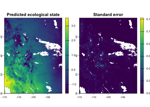

plot of chunk impact

The kernel and theta parameters control how analog influence decays with environmental distance. A Gaussian kernel with theta = 0.15 means analogs at an environmental dissimilarity distance of 0.15 receive about 60% weight, while those at 0.45 (= 3 × theta) receive almost none. The hard threshold max provides an absolute cutoff.

Spatial interpolation

The analog framework is also useful for analyses outside climate change scenarios. When x and pool share the same climate era, analog_impact() performs environmentally- and/or geographically-informed interpolation: for each grid cell, it finds sample locations with similar environment or nearby locations, then computes a weighted average of their measured values. This is useful for mapping ecological variables from sparse field observations onto a continuous grid. Unlike purely geographic interpolation methods (inverse distance weighting, kriging), this approach can also weight observations by environmental similarity, so a distant site with matching environment can contribute more than a nearby site with different environment.

The example below shows an interpolation informed by both climatic similarity and geographic proximity, with their relative importance determined by the theta parameters and the shape of the selected kernel function.

# Simulate sparse field observations at 500 random locations
set.seed(123)
n_sites <- 500
cells <- sample(which(!is.na(values(hist[[1]]))), n_sites)
sites <- as.data.frame(hist, xy = TRUE, na.rm = FALSE)[cells, ]
sites$observed <- 2 * sites$CWD - 0.5 * sites$AET + rnorm(n_sites, sd = 0.3)

# Interpolate onto the full grid
interp <- analog_impact(
      x = hist,
      pool = as.matrix(sites[, c("x", "y", "CWD", "AET")]),
      y = sites$observed,
      env = kernel(weight = "gaussian", theta = 0.15, max = 1),
      geog = kernel(weight = "gaussian", theta = 100, max = 200)
)

plot(interp[["weighted_mean"]], main = "Climate-informed spatial interpolation")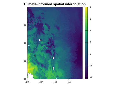

plot of chunk interpolation

Local regression

analog_regression() fits a weighted linear regression model within each analog neighborhood. This is useful if your outcome variable y has important relationships with additional predictors beyond the variables (env and geog) used to define the analog search kernel. In the example below we’ll use AET and its square as covariates. The function returns and returns the coefficients (and optionally, their standard errors) for each location in x, and also returns predicted values if x_covariates is provided.

The lambda parameter controls the amount of ridge regularization. The default (lambda = 0) is ordinary weighted least squares regression, with no regularization. Setting lambda > 0 adds regularization, which shrinks high-variance coefficients toward zero; this is useful for stabilizing predictions when some neighborhoods have few analogs relative to the number of covariates, or when covariates are strongly correlated. As lambda -> Inf, the intercept term approaches the weighted mean, i.e. the behavior of analog_impact(). The typical approach for choosing a lambda value is cross-validation (see the section on analog_cv() below), but here we’ll arbitrarily pick a modest value.

# Simulate covariates for the pool (just using AET for expediency)
set.seed(42)
pool_covariates <- data.frame(
      aet = as.vector(values(hist$AET)),
      aet2 = as.vector(values(hist$AET))^2
)

# Do the same for x (not required but enables predicted values)
x_covariates <- data.frame(
      aet = as.vector(values(fut$AET)),
      aet2 = as.vector(values(fut$AET))^2
)

# Fit analog regression model
fit <- analog_regression(
      x = fut,
      pool = hist,
      y = eco_var,
      covariates = pool_covariates,
      x_covariates = x_covariates,
      env = kernel(weight = "gaussian", theta = 0.15, max = 0.25),
      geog = kernel(max = 200),
      lambda = 1,
      se = "ess" # request standard errors
)

# Plot a few of the output variables
plot(fit[[c("coef_aet", "se_aet", "pred")]],
     main = c("A coefficient", "The coefficient's SE", "Predicted value"),
     nr = 1)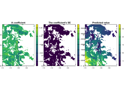

plot of chunk regression

Geographically weighted regression

The same regression machinery supports geographically weighted regression (GWR) by using geographic neighborhoods and geographic distance kernel weighting. This is a different configuration of the same underlying framework — no environmental constraint, geographic kernel, local regression on covariates.

# GWR: geographic neighborhood, geographic kernel weighting
gwr <- analog_regression(
      x = hist,
      pool = hist,
      y = eco_var,
      covariates = pool_covariates,
      select = "all",
      geog = kernel(weight = "inverse", theta = 30, max = 100),
      lambda = 0
)

plot(gwr[[c("coef_intercept", "coef_aet")]],
     main = c("GWR intercept", "GWR coefficient: cov1"),
     range = c(-2, 2), fill_range = TRUE)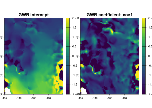

plot of chunk gwr

Cross-validation

Cross-validation (CV) is a technique that involves comparing observed data (y values for a given focal site) to predicted versions of those same values made using a model that was fit on a subset of the data that excludes the focal site. CV is useful for estimating prediction error on historical data (to understand uncertainty) and for calibrating model parameters (to improve predictive accuracy).

analog_cv() provides CV workflows for analog_impact() and analog_regression(). It runs an analog analysis in cross-validation mode and returns held-out predictions alongside observed values and residuals. You can plot and analyze CV results directly, or pass them to cv_performance() to calculate a basic set of overall performance metrics (e.g., R-squared for continuous outcomes, AUC for binary outcomes, etc.).

The CV routine supports leave-one-out (LOO), buffered LOO, and k-fold cross-validation methods. In contrast to traditional statistical models, LOO actually runs faster than k-fold for analog models because separate models are already being fit for each focal. Standard LOO (cv_method = "loo") is the default method, and excludes each focal site’s own data point from model fitting. Buffered LOO (cv_method = "loo", geog = kernel(min = ...)) excludes each focal site and all sites within a specified geographic distance, which can help mitigate over-optimistic performance measures resulting from spatial autocorrelation. K-fold cross-validation splits the data into a set of partitions, either randomly or based on groups you define, and excludes all points in each focal’s own partition during fitting.

Importantly, cross-validation is internal to pool—it does not take an x argument and can’t quantify how well the model predicts values in an independent dataset of focal sites. Thus it should not be assumed that CV performance metrics necessarily represent model transferability to data from different regimes (such as an x dataset representing future climates).

As an example, let’s run LOO cross-validation for an analog impact model, plot a map of the residuals, and quantify the model’s performance. If we wanted to tune a model parameter (labmda max_geog, theta, etc.), we could call cv_performance(analog_cv(...)) repeatedly with different parameter values to identify the best-performing settings.

# Run cross-validation and plot residuals
cv <- analog_cv(
      fun = analog_impact, pool = hist, y = eco_var,
      env = kernel(weight = "gaussian", theta = 0.15, max = .5),
      geog = kernel(weight = "gaussian", theta = 60, max = 200),
      se = "ess", cv_method = "loo"
)
plot(cv$residual, main = "Cross-validation residual")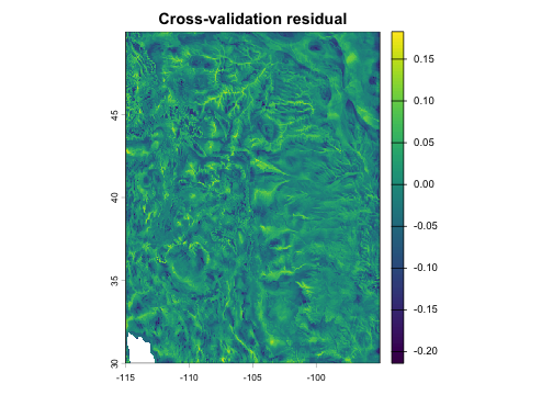

plot of chunk cv


# Calculate prediction error metrics
cv_performance(cv)
#>   variable       type metric         value
#> 1        y continuous      n  2.288230e+05
#> 2        y continuous   rmse  3.827635e-02
#> 3        y continuous    mae  2.946300e-02
#> 4        y continuous   bias -2.129624e-03
#> 5        y continuous     r2  9.985170e-01

Computational performance

The package is designed for large-scale analyses involving millions of pairwise comparisons.

Pre-built indices

When running multiple queries against the same reference pool, build the lattice index once and reuse it:

idx <- build_analog_index(hist)

# Multiple queries reuse the same index
avail_tight <- analog_availability(fut, idx, env = kernel(max = 0.3), geog = kernel(max = 100))
avail_loose <- analog_availability(fut, idx, env = kernel(max = 0.8), geog = kernel(max = 300))

Index tuning

By default, the lattice resolution is auto-tuned for each query. For repeated queries with the same configuration, you can tune once and reuse:

res <- tune_index_res(
      x = fut, pool = hist,
      stat = "count",
      env = kernel(max = 0.5), geog = kernel(max = 200),
      verbose = TRUE
)
idx <- build_analog_index(hist, index_res = res)

Parallel processing

Use the n_threads parameter to parallelize across focal locations:

result <- analog_velocity(fut, hist, env = kernel(0.5), k = 1, n_threads = 4)

Large raster datasets

For rasters too large to fit in memory, tiled_analog_search() processes the focal data in spatial tiles:

result <- tiled_analog_search(
      x = very_large_raster,
      pool = idx,
      stat = "count",
      env = kernel(max = 0.5),  
      geog = kernel(max = 200),
      n_tiles = 16
)

Downsampling

For very large reference pools, downsampling reduces computation. The package uses an adaptive sampling routine that reduces the effects on precision by downsampling more heavily in dense regions of environmental-geographic space in order to preserve coverage in sparse regions. As noted above, each pool site in the downsampled data gets a sample weight that’s used to correct summary statistics so that downsampling doesn’t bias the results:

result <- analog_availability(
      x = fut, 
      pool = hist,
      env = kernel(max = 0.5), 
      geog = kernel(max = 200),
      downsample = 0.1
)