Chiaroscuro

[VISUALIZATION] Animating shifting sunlight over complex terrain.

A lot of our research in the Ackerly lab is focused on understanding how climate variation shapes plant ecology, and one key driver of climate is local topography. In the northern hemisphere, higher radiation loads make south-facing slopes much warmer and drier on average—but solar radiation varies based on latitude, season, and time of day, as well as the topographic slope and aspect of a given site. Partly just as an excuse to play with the new rayshader package, I thought I’d take a stab at creatting a realistic sunlight animation for Pepperwood Preserve, a site in the California coast ranges where our lab does extensive long-term forest monitoring research.

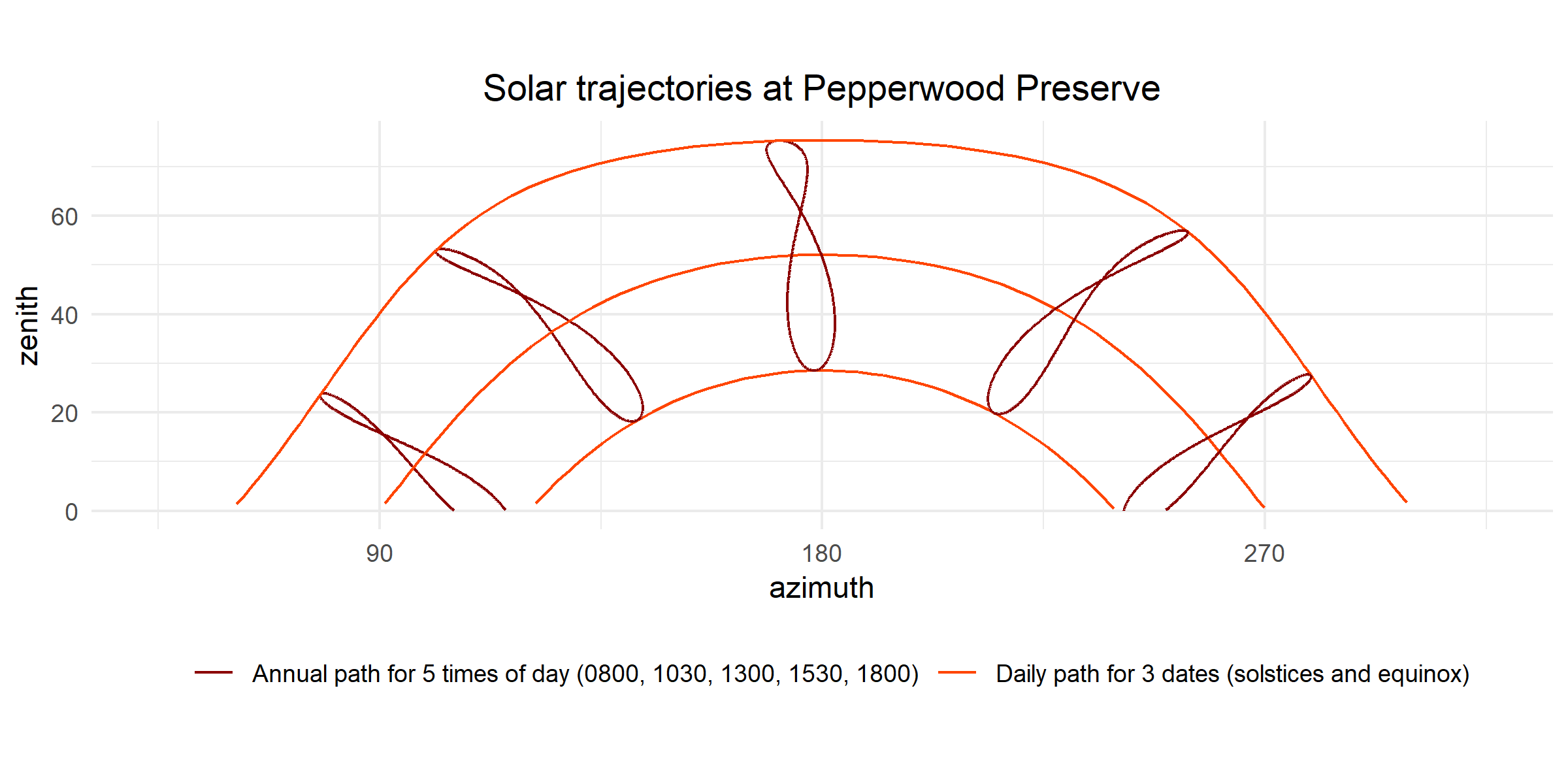
Rayshader provides a set of tools to generate beautiful and realistic hillshaded graphics from digital elevation data. The package lets you specify any arbitrary sun position, but I wanted to use use the sun’s real trajectory across the sky. For this I turned to the insol package, which we can use to compute the exact azimuth and zenith of the sun based on a date, time of day, and geographic coordintes. Here is some solar position data for Pepperwood, showing the swath of sky traversed by the sun at different times of year here in central California:

The lower line shows the sun’s daily path on the winter solstice. To animate how landscape lighting at Pepperwood evolves over the course of the solstice, we can generate a set of sun points along the line, use rayshader in combination with some high-resolution elevation data to generate a hillshade image for each sun point, and then stitch the frames together into a gif using the magick package. This gives us the visualization at the top of the post. Pretty fun what you can do with just a few lines of R code these days! The core code is just the folowing:

# load packages
library(tidyverse)
library(raster)
library(insol)
library(magick)
library(rayshader)

# load elevation data
elmat <- raster("dem.tif") %>% as.matrix() %>% t()
zscale <- 10 # ratio of pixel resolution (10m) to elevation unit (m)

# generate a sequence of solar positions
sp <- seq(ISOdate(2012,12,20,0), ISOdate(2012,12,20,24), by="min") %>%
      JD() %>%
      sunvector(38,-122,-7) %>% # lat, long, time zone at Pepperwood
      sunpos() %>% 
      as.data.frame() %>%
      mutate(id = 1:nrow(.),
             zenith = 90-zenith) %>%
      filter(zenith >= -10, # exclue nighttime
             id %% 3 == 0) # keep every third frame

# open magick graphics device
img <- image_graph(width=500, height=500)

# generate hillshade image for each solar position
for(i in 1:nrow(sp)){
      azimuth <- sp$azimuth[i]
      zenith <- sp$zenith[i]
      
      texture <- create_texture("red", "darkgreen",
                                "khaki", "khaki", "khaki")
      
      elmat %>%
            sphere_shade(texture=texture, sunangle=azimuth, zscale=zscale) %>% 
            add_shadow(ambient_shade(elmat, zscale=zscale)) %>%
            add_shadow(ray_shade(elmat,
                                 anglebreaks=seq(zenith-4, zenith+4, 1),
                                 sunangle=azimuth, zscale=zscale),
                       max_darken=.3) %>%
            plot_map()
}

# save animation
dev.off()
img %>% image_animate(fps = 10) %>% image_write("animation.gif")