Particle trails

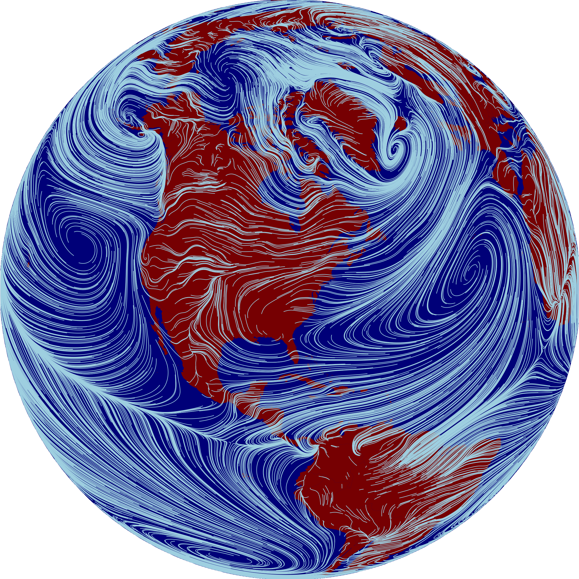
[VISUALIZATION] Illustrating the geography of wind and climate change.

I just returned from a fantastic trip to the Species on the Move conference in South Africa, where I presented some work focused on relationships between wind patterns and biodiversity migration under climate change. I got a number of inquiries from folks about the wind and temperature gradient visualizations I showed in my talk, so thought I’d do a quick demo here of how I created those in R.

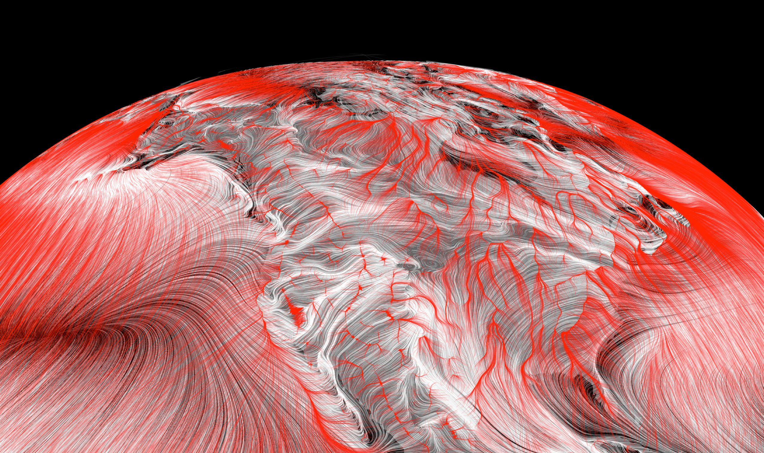
The figure above illustrates prevailing near-surface winds by showing the paths that wind-blown particles would follow. Full credit for the inspiration goes to the gorgeous wind maps at hint.fm. What’s fun is we can use the same style to visualize trails that climate-tracking species ranges might follow, by sending particles down local temeperature gradients rather then downwind – that’s illustrated in red in the figure of North America below, overlaid on wind paths in white. The temperature trails clearly follow latitudinal gradients in eastern North America, while in the west they follow elevational gradients toward the ridgelines of major mountain ranges.

For all these figures, the data input is a vector field, i.e. a grid of eastward and northward speeds. We initialize a bunch of particles in random places across the grid, and then simulate their movement by nudging their positions according to nearby values in the vector field. The resulting trails can be overlaid in sill images like the ones here, or used to build animations like these by Cameron Beccario. Here’s some code showing how to reproduce the global wind figure above:

# load libraries
library(raster)
library(tidyverse)

# latitude-based adjustment factor to correct for geodesic distortion
distortion <- function(lat){
      x <- geosphere::distGeo(c(0, lat), c(.0001, lat))
      y <- geosphere::distGeo(c(0, lat), c(0, lat - sign(lat) * .0001))
      y / x
}

# function to simulate particle trails from a vector field
particle_trails <- function(d, # vector field rasters
                            np, # number of particles
                            nt, # number of timesteps
                            r, # smoothing neighborhood radius
                            scale){ # multiplier converting velocity to lat-lon
      
      x <- sort(unique(coordinates(d)[,1]))
      y <- desc(sort(unique(coordinates(d)[,2])))
      dx <- as.matrix(d[[1]])
      dy <- as.matrix(d[[2]])
      distort <- sapply(y, distortion)
      
      ptx <- pty <- matrix(NA, nt, np)
      for(p in 1:np){
            px <- runif(1, min(x), max(x))
            py <- runif(1, min(y), max(y))
            
            for(t in 1:nt){
                  xi <- which(x > px - r & x < px + r)
                  yi <- which(y > py - r & y < py + r)
                  
                  px <- px + mean(dx[yi, xi]) * scale * mean(distort[yi])
                  py <- py + mean(dy[yi, xi]) * scale
                  
                  ptx[t, p] <- px
                  pty[t, p] <- py
                  
                  if(py > 90 | py < -90) break()
                  if(px > 180) px <- px - 360
                  if(px < -180) px <- px + 360
            }
      }
      
      frame <- function(pd){
            colnames(pd) <- paste0("p", 1:ncol(pd))
            as.data.frame(pd) %>%
                  mutate(time = 1:nrow(.)) %>%
                  gather(id, z, -time)
      }
      
      left_join(frame(ptx) %>% rename(x = z),
                frame(pty) %>% rename(y = z))
}

# load raster dataset with 2 layers: 
#     zonal and meiridional windspeeds
# and simulate particle trails
w <- stack("wind_uv.tif")
f <- particle_trails(d = w, np = 10000, nt = 100, r = 1, scale = .1)

# continent and ocean data
continents <- map_data("world")
ocean <- ocean0 <- data.frame(x=c(rep(0, 100), rep(10, 100)),
                        y=c(seq(-90, 90, length.out=100),
                            seq(90, -90, length.out=100)),
                        group=1)
for(i in 1:360) ocean <- bind_rows(ocean, mutate(ocean0, x=x+i, group=i))

# the plot, with an ortho projection
ggplot() +
      geom_polygon(data=ocean, aes(x, y, group=group),
                   fill="darkblue", color="darkblue") +
      geom_polygon(data=continents, aes(long, lat, group=group),
                   fill="darkred") +
      geom_path(data=f %>% filter(x>-180, x<180),
                aes(x, y, group=id),
                color="lightblue", size=.25) +
      coord_map("ortho", orientation = c(40, -82, 0)) +
      theme_void() +
      theme(legend.position="none")